
A set of Matlab software demonstrations of particle filtering for tracking applications, developed in the context of lectures given from 2005 to 2013:
- SAGEM, Argenteuil — 12–13 juin, 3–4 juillet, 19 septembre. 2003 [slides],
- Centre de Compétence Technique (CCT) et Centre National d’\’Etudes Spatiales (CNES) Toulouse, Novembre 24, 2003,
- École Chercheurs en “traitement du signal”, Inria Rennes, 18 au 20 octobre 2004,
- IAP DYSCO Study Day, Dynamical systems, control and optimization – University of Louvain, Mons. Friday May 24, 2013 [slides],
and in many seminars and in doctoral training programs. I also used these Matlab software demonstrations in a course I taught in Toulon from 2004 to 2008 as part of the Master of Science and Technology at the University of the South Toulon-Var [pdf, the 2006 version if in the CEL website here].
See gitlab repository.
The code has been registered in 2009 at the Agence pour la Protection des Programmes (APP) [reference IDDN.FR.001.28003.000.S.P.2009.000.31235].
SMC are a class of algorithms for approximate inference in dynamic models. They are used to estimate the state of a system over time, given a sequence of noisy measurements. The basic idea of SMC methods is to represent the probability distribution over the state of the system at each time step using a set of weighted samples, or particles. The particles are propagated through time using the dynamics of the system, and their weights are updated based on the measurements that are made. The weights are used to approximate the true distribution, and they can be used to compute various statistics of interest, such as the mean and covariance of the state. SMC methods are useful because they allow us to make inferences about the state of a system in a computationally efficient manner, without requiring us to compute the true distribution explicitly. They have been applied in many fields.
Context
In all these examples a mobile is describe by its state  in
in  at time
  which is a Markov process described by a Markov transition kernel
  with:
with:
![\[ Q_t(x,A) = \mathbb{P}(X_t\in A|X_0=x) \]](../../wp-content/ql-cache/quicklatex.com-9317f06167a117ddd3fe3361d1584ecb_l3.png "Rendered by QuickLaTeX.com")
for example it could be given by an SDE
![\[ d X_t = f(X_t)\,dt + g(X_t)\,dB_t \]](../../wp-content/ql-cache/quicklatex.com-5a124d36e8fa2a3f3a6a265d52967994_l3.png "Rendered by QuickLaTeX.com")
The observation process is  which is the observation of at time
  given by:
![\[ Y_k = h(X_{t_k})+\textrm{observation noise} \]](../../wp-content/ql-cache/quicklatex.com-f1736859f16353bc4060f33f6de29d6d_l3.png "Rendered by QuickLaTeX.com")
with  .
.
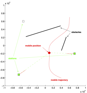
Target tracking with angle only and obstacles
The original idea for this very nice example came from Simon Maskell.
The idea is to follow a mobile on the plane. We have  observation stations (squares) and
  obstacles (black segments) that hide the movement of the mobile.
The measures are the angle of the line of sight plus noise.
In the video, we place 1) the observations stations, 2) the obstacles, then 3) we plot the trajectory of the mobile, and 4) we simulate the observations, finally 5) we plot the evolution of the particles of the approximation of the nonlinear filter.
We notice the ability of the particle filter to handle non Gaussian situations.
A mobile in Manhattan
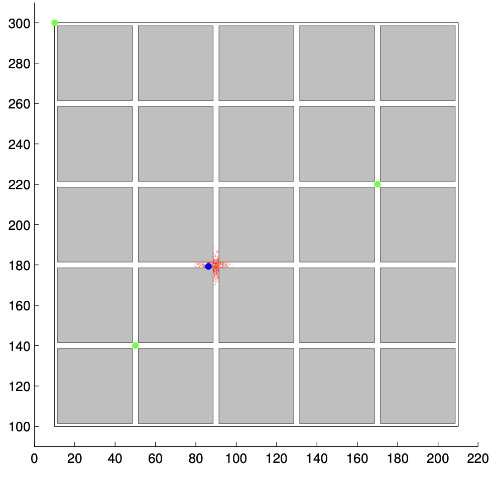
It is about geolocating a mobile, a person using a cell phone, in a simplified Manhattan. The mobile can move in the street (white zone) or in the buildings (grey zones).
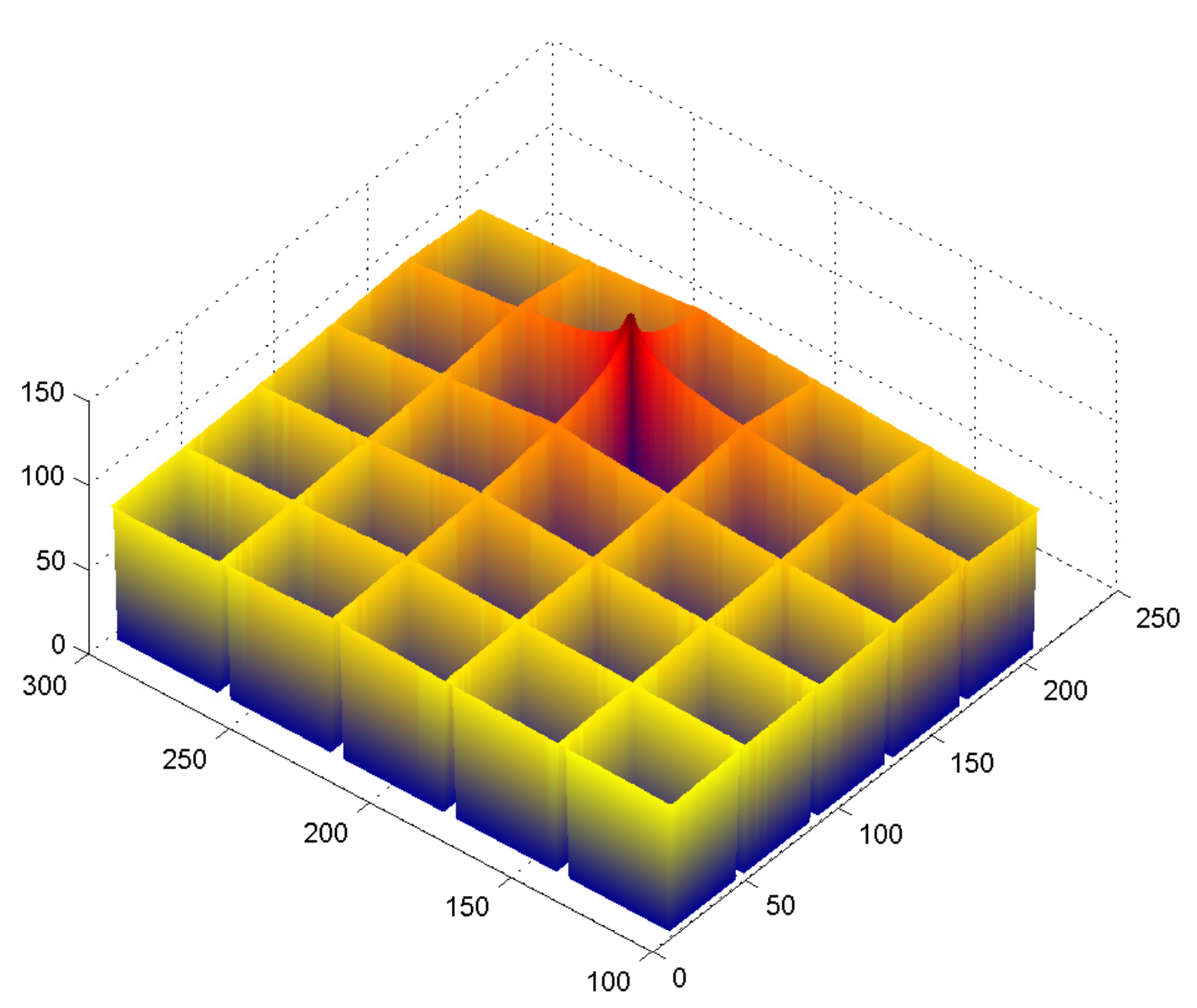
The area is covered by several antennas represented by green dots. To each of these antennas corresponds an attenuation map (bottom figure). This map describes in each point of the area the attenuation of the signal transmitted by the mobile and received by the antenna. In this simplified version it is assumed that this signal is zero
when the mobile is in a building, and that it decreases when the mobile moves away from the antenna.
In the following video we position the antennas (green dots) and then we define the trajectory of the mobile: it can move in the street or in buildings.