INRIA home page
Subsections
The purpose of this chapter is to describe the methods based on
interval analysis available in the ALIAS library for the
determination of real roots of
system of equations and inequalities.
Interval Analysis
This section is freely inspired from the book [5].
An interval number is a real, closed interval
 . Arithmetic
rules exist for interval numbers. For example let two interval numbers
. Arithmetic
rules exist for interval numbers. For example let two interval numbers
 ,
,
 , then:
An interval function is an interval-valued function of one or
more interval arguments. An interval function  is said to be inclusion monotonic if
 for
for  in
in ![$[1,n]$](img11.png) implies:
implies:
A fundamental theorem is that any rational interval function evaluated
with a fixed sequence of operations involving only addition,
subtraction, multiplication and division is inclusion monotonic.
This means in practice that the interval evaluation
of a function gives bounds (very often overestimated) for the value of
the function: for any specific values of the unknowns within their
range the value of the function for these values will be included in
the interval evaluation of the function. A very interesting point is
that the above statement will be true even taking into account
numerical errors. For example the number 1/3, which has no exact
representation in a computer, will be represented by an interval
(whose bounds are the highest floating point number less than 1/3 and
the smallest the lowest floating point number greater than 1/3) in
such way that the multiplication of this interval by 3 will include
the value 1. A straightforward consequence is that if the interval
evaluation of a function does not include 0, then there is no root of
the function within the ranges for the unknowns.
In all the following sections an interval for the variable  will be
denoted by
. The width or diameter of an interval
is the
positive difference
will be
denoted by
. The width or diameter of an interval
is the
positive difference
 .
The mid-point of an interval is defined as
.
The mid-point of an interval is defined as
 .
.
A box
is a set of intervals. The width of a box is the largest width of the
intervals in the set and the center of the box is the vector
constituted with the mid-point of all the intervals in the set.
Implementation
All the procedures described in the following sections use the free
interval analysis package
BIAS/Profil
in which the basic operations of interval
analysis are implemented2.1.
This package uses a fixed precision arithmetics with an accuracy of
roughly  .
Different types of data structure are implemented in this package. For
fixed value number:
.
Different types of data structure are implemented in this package. For
fixed value number:
BOOL, BOOL_VECTOR, BOOL_MATRIX,
INT, INTEGER_VECTOR, INTEGER_MATRIX, REAL, VECTOR, MATRIX, COMPLEX
for intervals:
INTERVAL, INTERVAL_VECTOR, INTERVAL_MATRIX
All basic arithmetic operations can be used on interval-valued data
using the same notation than for fixed numbers. Not that for vector
and matrices the index start at 1:  for an interval matrix
represents the interval at the first row and first column of the
interval matrix
for an interval matrix
represents the interval at the first row and first column of the
interval matrix  . The type INTERVAL_VECTOR will be used to
implement the box concept, while the type INTERVAL_MATRIX will
be used to implement the concept of list of boxes.
. The type INTERVAL_VECTOR will be used to
implement the box concept, while the type INTERVAL_MATRIX will
be used to implement the concept of list of boxes.
For the evaluation of more complex interval-valued function there are
also equivalent function in the BIAS/Profil, whose name is usually
obtained from their equivalent in the C language by substituting their
first letter by the equivalent upper-case letter: for example the
evaluation of  where
where  is an interval will be obtained by
calling the function
is an interval will be obtained by
calling the function  . We have also introduced in ALIAS
some other mathematical operators whose names are derived from their
Maple implementation: ceil, floor, round.
. We have also introduced in ALIAS
some other mathematical operators whose names are derived from their
Maple implementation: ceil, floor, round.
Table 2.1 indicates the
substitution for the most used functions.
Table 2.1:
Equivalent interval-valued function
| C function |
Substitution |
C function |
Substitution |
| sin |
Sin |
cos |
Cos |
| tan |
Tan |
arcsin |
ArcSin |
| arccos |
ArcCos |
arctan |
ArcTan |
| sinh |
Sinh |
cosh |
Cosh |
| tanh |
Tanh |
arcsinh |
ArcSinh |
| arccosh |
ArcCosh |
arctanh |
ArcTanh |
| exp |
Exp |
log |
Log |
| log10 |
Log10 |
 |
Sqr |
| sqrt |
Sqrt(x) |
$](img23.png) |
Root(x,i) |
 |
Power(x,i) |
 |
Power(x,y) |
 |
IAbs(x) |
ceil() |
ALIAS_Ceil() |
| floor() |
ALIAS_Floor() |
rint() |
ALIAS_Round() |
|
Note also that the mathematical operators  ,
,  ,
,
 exist under the name Cot, ArcCot, ArCoth.
A special operator is defined in the procedure ALIAS_Signum:
formally it defines the signum operator of Maple defined as
which is not defined at  . In our implementation for an interval
![$x =[\underline{x},\overline{x}]$](img32.png) ALIAS_Signum() will
return:
ALIAS_Signum() will
return:
- $$
- 1if

- $$
- -1 if

- $$
- 1if is lower than ALIAS_Value_Sign_Signum and
ALIAS_Sign_Signum is positive
- $$
- -1 if is lower than ALIAS_Value_Sign_Signum and
ALIAS_Sign_Signum is negative
- -1,1
- otherwise
The default value for ALIAS_Value_Sign_Signum and
ALIAS_Sign_Signum are respectively 1e-6 and 0.
The derivative of ALIAS_Signum is defined in the procedure
ALIAS_Diff_Signum.
Formally this derivative is 0 for any not equal to 0. In our
implementation ALIAS_Diff_Signum() will return 0 except if
is lower than ALIAS_Value_Sign_Signum in which case the
procedure returns [-1e11,1e11].
The derivative of the absolute value is defined in the procedure
ALIAS_Diff_Abs.
If the interval X includes 0 the procedure returns [-1e11,1e11]
otherwise it returns ALIAS_Signum(X).
Using the above procedures
when an user has to write an interval-valued function he has to
convert its C source code using the defined substitution. For example
if a function is written in C as:
then its equivalent interval valued function is
A special care has to be used when transforming an equation into its
interval equivalent. The formulation may play a role in the
efficiency. For example you should avoid as much as possible multiple
occurences of the same variable as this will usually lead to an
overestimation of the interval evaluation. For example  is
better written as
is
better written as  . You should also avoid as much as possible
to repeat the same evaluation. For example if an expression is
involved several times in equation(s) you better have to assign once the
interval evaluation of this expression in a temporary interval
variable and use this variables in the calculation.
Transforming equation in their interval equilvalent is a tedious
process and may be automated using the ALIAS-Maple procedure
MakeF that produces automatically the C++ code and apply
heuristics for obtaining the most efficient form. There is another
procedure MakeJ that will produce automaticaaly the code for the gradient
matrix being given the equations and variables.
. You should also avoid as much as possible
to repeat the same evaluation. For example if an expression is
involved several times in equation(s) you better have to assign once the
interval evaluation of this expression in a temporary interval
variable and use this variables in the calculation.
Transforming equation in their interval equilvalent is a tedious
process and may be automated using the ALIAS-Maple procedure
MakeF that produces automatically the C++ code and apply
heuristics for obtaining the most efficient form. There is another
procedure MakeJ that will produce automaticaaly the code for the gradient
matrix being given the equations and variables.
Note that all the even powers of an interval are better managed with
the Sqr and Power procedures. Indeed let consider the
interval ![$X=[-1,1]$](img39.png) , then the interval product
, then the interval product  leads to the
interval [-1,1] while the interval Sqr() leads to [0,1].
For an interval
the width of the interval is obtained by
using the procedure Diam() while we have
leads to the
interval [-1,1] while the interval Sqr() leads to [0,1].
For an interval
the width of the interval is obtained by
using the procedure Diam() while we have
 Inf() and
  Sup().
We will denote by box a set of intervals which
define the possible values of the unknowns. By extension and according
to the context boxes may also be used to denote a set
of such set. A function intervals will denote the
interval values of a set of functions for a given box,
while a solution intervals will denote the box which
are considered to be solution of a system of functions.
Problems with the interval-valuation of an expression
An important point is that not all expressions can be evaluated using
interval arithmetics. Namely constraints that prohibits the interval
evaluation of an expression are:
- denominator that may include 0
- argument of square should be positive
- argument of arcsin and arccos should be included in [-1,1]
- argument of log,ln,log10 should be positive
- argument of arccosh should be greater than 1
- argument of arctanh cannot include the interval [-1,1]
- argument of where
 is not an integer should be positive
- argument of
 should not be too large to avoid
overflow problem.
should not be too large to avoid
overflow problem.
If such situation occurs a fatal error will be generated at run time.
Hence such special cases has to be dealt with carefully.
ALIAS-Maple offers the possibility of dealing with such problem. For
example the procedure Problem_Expression allows one to
determine what constraints should be satisfied by the unknowns so that
each equations can be interval evaluated, see the ALIAS-Maple documentation.
If you use your own evaluation procedure and are
aware of evaluation problems and modify the returned values if such
case occurs it will be
a good policy to set C++ flags ALIAS_ChangeF, ALIAS_ChangeJ to 1 (default value 0) if a change occurs.
Currently the interval Newton scheme that is embedded in some of the
solving procedures of ALIAS will not be used if one of these
flags is set to 1 during the calculation.
In some specific cases we may have to deal with interval in which
infinity is used. These quantities are represented using BIAS
convention, BiasNegInf representing the negative infinity and
BiasPosInf the positive infinity.
Non 0-dimensional system
Although the solving procedures of ALIAS are
mostly devoted to be used for 0 dimensional system
(i.e. systems having a finite number of solutions) most of them can
still be used for non 0-dimensional system. In that case the result
will be a set of boxes which will be an approximation of the
solution. When dealing with such system it is necessary to set the
global variable ALIAS_ND to 1 (its default value is 0) and to
define a name in the character string ALIAS_ND_File. The
solution boxes of the system will be stored in a file with the
given name.
The quality of the approximation may be estimated with the flags
ALIAS_Volume_In, ALIAS_Volume_Neglected that give
respectively the total volume of the solution boxes and the total
volume of the neglected boxes (i.e. the boxes for which the algorithm
has not been able to determine if they are or not a solution of the
system).
Note that there are special procedures for 1-dimensional system, see
chapter 9.
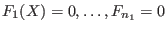
General purpose solving algorithm
This algorithm enable to determine approximately the solutions of a
system of  equations and inequalities
in
equations and inequalities
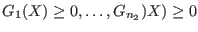
in  unknowns. Hence this method may be used to solve
a system
composed of
unknowns. Hence this method may be used to solve
a system
composed of  equations
 ,
,  inequalities
 and
and  inequalities
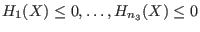 .
.
Let
 be the set of unknowns and
let
be the set of unknowns and
let
 be the set of
  intervals in which you are searching the solutions
of the
intervals in which you are searching the solutions
of the  equations
 (for the sake of simplicity we don't consider
inequalities but the extension to inequalities is straightforward).
(for the sake of simplicity we don't consider
inequalities but the extension to inequalities is straightforward).
We will denote by  the interval value of
  when this
function is evaluated for the box
when this
function is evaluated for the box
 of the unknowns while
  will denote the
-dimensional interval vector constituted of the when the
unknowns have the interval value defined by the set
will denote the
-dimensional interval vector constituted of the when the
unknowns have the interval value defined by the set  .
.
The algorithm will use a list of boxes  whose maximal size
  is an
input of the program. This list is initialized with
is an
input of the program. This list is initialized with  . The
number of currently in the list is
. The
number of currently in the list is  and therefore at the
start of the program
and therefore at the
start of the program  . The algorithm will also use an accuracy on
the variable
. The algorithm will also use an accuracy on
the variable  and on the functions
  . The norm of a is defined as:
The norm of the interval vector is defined as:
The algorithm uses an index and the result is a
set  of interval vector
  for the unknowns whose size is
  .
We assume that there is no
.
We assume that there is no  with
with  in such that
 or
or
 ,
otherwise the equations have no solution in .
Two lists of interval vectors
,
otherwise the equations have no solution in .
Two lists of interval vectors
 whose size
is
whose size
is  will also be used.
The algorithm is initialized with
will also be used.
The algorithm is initialized with  and proceed along the following steps:
- if
 return
  and and exit
- bisect
 which produce new interval vectors
 and set
- for

- evaluate

- if it exist with in such that
 or
or
 ,
then
,
then
 and go to step 3
- if
 or
or
 , then store in
  , increment and go to step 3
- store in
 , increment
  and go
to step 3
and go
to step 3
- if increment and go to step 1
- if
 return a failure code as there is no space
available to store the new intervals
return a failure code as there is no space
available to store the new intervals
- if
 store one of the
  in , the other
 at the end of , starting at position
  . Add
to and go to step 1
. Add
to and go to step 1
Basically the algorithm just bisect the box until either
their width is lower than or the width of the interval
function is lower than  (provided that there is enough
space in the list to store the intervals). Then if all the intervals
functions contain 0 we get a new solution, if one of them does not
contain 0 there is no solution of the
equations within the current box. A special case occurs
when all the components of the box are reduced to a point, in which case a
solution is obtained if the absolute value of the interval evaluation
of the function is lower than .
(provided that there is enough
space in the list to store the intervals). Then if all the intervals
functions contain 0 we get a new solution, if one of them does not
contain 0 there is no solution of the
equations within the current box. A special case occurs
when all the components of the box are reduced to a point, in which case a
solution is obtained if the absolute value of the interval evaluation
of the function is lower than .
Now three problems have to be dealt with:
- how to choose the which will be put in place of the
and in which order to store the other at the
end of the list?
- can we improve the management of the bisection process in order
to conclude the algorithm with a limited number ?
- how do we distinguish distinct solutions ?
The first two problems will be addressed in the next section.
Managing the bisection and ordering
The second problem is solved in the following way: assume that at some
step of the algorithm the bisection process leads to the creation of
such that  . As we have previously considered the
 elements of we may use them as storage space. This
means that we will store
elements of we may use them as storage space. This
means that we will store
 at
at
 thereby freeing elements. In that case the procedure will fail
only if
thereby freeing elements. In that case the procedure will fail
only if  .
.
Now we have to manage the ordering of the . We have defined
two types of order for a given set of boxes :
- maximum equation ordering: the box are ordered
along the value of
 for
all in [1,]. The first box will have the lowest
for
all in [1,]. The first box will have the lowest  .
.
- maximum middle-point equation ordering: let
 be the
vector whose components are the middle points of the intervals .
The box are ordered
along the value of
be the
vector whose components are the middle points of the intervals .
The box are ordered
along the value of
 for
all in [1,]. The first box will have the lowest .
for
all in [1,]. The first box will have the lowest .
When adding the we will substitute the by the
having the lowest while the others will be
added to the list by increasing order of .
The purpose of these ordering is to try to consider first the
box
having the highest probability of containing a solution.
This ordering may have an importance in the determination of the
solution intervals (see for example section 2.3.5.2).
This method of managing the bisection is called the
Direct Storage mode and is the default mode in ALIAS. But
there is another mode, called the Reverse Storage
mode.
In
this mode we still substitute the by the
having the lowest but instead of adding the remaining
at the end of the list we shift by the
boxes in the list, thereby freeing the storage of
 which is used to store the remaining
. In other words we may consider the solving procedure as
finding a leaves in a tree which are solutions of the problem: in the
Direct Storage mode we may jump during the bisection from one
branch of the tree to another while in the Reverse storage mode
we examine all the leaves issued from a branch of
the tree before examining the other branches of the tree. If we are
looking for all the solutions the storage mode has no influence on the
total number of boxes that will be examined. But the Reverse
Storage mode may have two advantages:
which is used to store the remaining
. In other words we may consider the solving procedure as
finding a leaves in a tree which are solutions of the problem: in the
Direct Storage mode we may jump during the bisection from one
branch of the tree to another while in the Reverse storage mode
we examine all the leaves issued from a branch of
the tree before examining the other branches of the tree. If we are
looking for all the solutions the storage mode has no influence on the
total number of boxes that will be examined. But the Reverse
Storage mode may have two advantages:
- if we are looking for only one solution it may enable to find it
more rapidly (but that is not compulsory, see section 2.3.5.4),
- as we are following one branch at a time we will consider very
rapidly small box that either will lead to a solution or
will be discarded thereby enabling to free some storage space. Hence
the storage space available in the reverse mode will be in general
higher than in the direct mode: a practical consequence is that a
problem may not be solved with the direct mode due to problem in the
storage while with the same amount of storage solutions will be
obtained in the reverse mode.
To switch the storage mode see section 2.3.4.5 .We may also
define a mixed strategy which is staring in the direct mode and then
switching to the reverse mode when the storage becomes a problem (see
section 8.3).
An alternative: the single bisection
A possibility to reduce the combinatorial explosion of the previous
algorithm is to bisect not all the variables i.e. to use the
full bisection mode, but only one of
them (it must be noted that the algorithms in ALIAS will not
accept a full bisection mode if the number of unknowns exceed
10). This may reduce the computation time as the number of function
evaluation may be reduced. But the problem is to determine which
variable should be bisected. All the solving algorithms of ALIAS
may manage this single bisection by setting the flag Single_Bisection to a value different from 0.
The value of this global variable indicates various bisection modes.
Although the behavior of the
mode may change according to the algorithm here are the
possible modes for the general solving algorithm and the corresponding
values for Single_Bisection:
- 1 : we just split the variable having
the largest width (valid for all algorithms). Note however that it is
still possible to order the bisection i.e. to split first a subset of
the unknowns until their width is small (i.e. lower than
ALIAS_Accuracy, then another subset and so
on. This is obtained by setting flag
ALIAS_Ordered_Bisection
to 1 and
defining an integer matrix ALIAS_Order_Bisection
whose rows
indicate the bisected subset and
should end by 0. For example if this matrix has as rows
[1,3,0],[2,4,5,0], then the algorithm will first bisect the unknowns 1
and 3 until their width is small, then the unknowns 2,4,5. If all
unknowns indicated in the rows of the matrix have a small width, then
the bisection algorithm revert to the normal behavior.
- 2: to determine the variable that will be bisected we use the following
approach: we compute the order criteria for the two boxes
 that will result from the bisection of variable
  and retain the lowest
criteria
and retain the lowest
criteria  . The variable that will be bisected is the one that has the
lowest except if for at least one variable the interval
evaluation of the function for
. The variable that will be bisected is the one that has the
lowest except if for at least one variable the interval
evaluation of the function for  or
or  does not contain 0. In
that case the variable that will be bisected is the one that
verify the previous property and which has the lowest among all
the input intervals having the property.
However to avoid bisecting over and over
the same variable we use another test: let
does not contain 0. In
that case the variable that will be bisected is the one that
verify the previous property and which has the lowest among all
the input intervals having the property.
However to avoid bisecting over and over
the same variable we use another test: let  be the width of the
interval
be the width of the
interval
![$[\underline{x_i},\overline{x_i}]$](img118.png) and
and  be the
maximum of all the . If
be the
maximum of all the . If
 we don't consider the
variable as a possible bisection direction.
It is also possible to mix this mode with mode 1. If the integer
variable ALIAS_RANDG is set to a strictly positive value then
ALIAS_RANDG bisection will be performed using mode 2 while the
next bisection will be performed using mode 1 and the process will be
repeated
we don't consider the
variable as a possible bisection direction.
It is also possible to mix this mode with mode 1. If the integer
variable ALIAS_RANDG is set to a strictly positive value then
ALIAS_RANDG bisection will be performed using mode 2 while the
next bisection will be performed using mode 1 and the process will be
repeated
- 3, 4 : similar to 1
- 5 : we use a round-robin mode i.e. each variable is
bisected in turn (first
 , then
  and so on) unless the width
of the input intervals is less than the desired accuracy on the
variable, in which case the bisected variable is the next one having a
sufficient width (valid for all algorithms)
The flag ALIAS_Round_Robin is used to indicate at each
bisection which variable should be bisected.
and so on) unless the width
of the input intervals is less than the desired accuracy on the
variable, in which case the bisected variable is the next one having a
sufficient width (valid for all algorithms)
The flag ALIAS_Round_Robin is used to indicate at each
bisection which variable should be bisected.
- 6: we emulate the smear function (see section 2.4.1.3)
with an estimation of the
gradient based on finite difference (procedure
Select_Best_Direction_Grad)
- 7: here again we use the flag
ALIAS_Ordered_Bisection
set to 1 and
defining an integer matrix ALIAS_Order_Bisection
whose rows indicates an order for bisecting the unknowns. The largest
variable in the first row will be bisected first and so on until all
the variables in a row have a width lower than
ALIAS_Accuracy. We then proceed to the second row.
As soon as all variables in all rows have a width lower than
ALIAS_Accuracy we use the bisection 1.
- 20: the user has defined its own bisection procedure, see
section 11.3
For all general purpose solving procedures the number of the variable
that has been
bisected is available in the integer
ALIAS_Selected_For_Bisection.
There is another mode called the mixed bisection: among the
variables we will bisect  variables, which will lead to
 new boxes. This mode is obtained by setting
the global integer variable
new boxes. This mode is obtained by setting
the global integer variable
ALIAS_Mixed_Bisection
to  . Whatever is the value of
Single_Bisection we will order the variables according to their width
and select the variables having the largest width.
. Whatever is the value of
Single_Bisection we will order the variables according to their width
and select the variables having the largest width.
An interval will be considered as a solution for a function
of the system in the following cases:
- for equations the maximal diameter of the intervals is less than
a given threshold epsilon and the corresponding interval
evaluation of the function contains 0 or the corresponding interval
evaluation of the function has a diameter less than a given threshold
epsilonf and the interval contains 0
- for inequalities
 : the upper bound of
the interval evaluation of the
function is negative or the maximal diameter of the
intervals is less than
a given threshold epsilon and the corresponding interval
evaluation of the function has at least a negative lower bound or the corresponding interval
evaluation of the function has a diameter less than a given threshold
epsilonf and the interval contains 0
: the upper bound of
the interval evaluation of the
function is negative or the maximal diameter of the
intervals is less than
a given threshold epsilon and the corresponding interval
evaluation of the function has at least a negative lower bound or the corresponding interval
evaluation of the function has a diameter less than a given threshold
epsilonf and the interval contains 0
- for inequalities
 : the lower bound of
the interval evaluation of the
function is positive or the maximal diameter of the
intervals is less than
a given threshold epsilon and the corresponding interval
evaluation of the function has at least a positive upper bound or the corresponding interval
evaluation of the function has a diameter less than a given threshold
epsilonf and the interval contains 0
: the lower bound of
the interval evaluation of the
function is positive or the maximal diameter of the
intervals is less than
a given threshold epsilon and the corresponding interval
evaluation of the function has at least a positive upper bound or the corresponding interval
evaluation of the function has a diameter less than a given threshold
epsilonf and the interval contains 0
A solution of the system is defined as a box such that
the above conditions hold for each function of the system.
Note that for systems having interval coefficients (which are
indicated by setting the flag ALIAS_Func_Has_Interval to 1)
a solution of a system will be obtained only if the inequalities are
strictly verified.
Assume that two solutions
 have been found
with the algorithm.
We will first consider the case where we have to solve a system of
equations in unknowns, possible with additional inequality
constraints.
First we will check with the Miranda theorem (see
section 3.1.5) if
include one (or
more) solution(s). If both solutions are Miranda, then they will kept
as solutions. If one of them is Miranda and other one is not Miranda
we will consider the distance between the mid-point of
: if this distance is lower than a given threshold we will
keep as solution only the Miranda's one. If none of
is Miranda we keep these solutions, provided that their distance
is greater than the threshold. Note that in that case these solutions
may disappear if a Miranda solution is found later on such that the
distance between these solutions and the Miranda's one is lower than
the threshold.
have been found
with the algorithm.
We will first consider the case where we have to solve a system of
equations in unknowns, possible with additional inequality
constraints.
First we will check with the Miranda theorem (see
section 3.1.5) if
include one (or
more) solution(s). If both solutions are Miranda, then they will kept
as solutions. If one of them is Miranda and other one is not Miranda
we will consider the distance between the mid-point of
: if this distance is lower than a given threshold we will
keep as solution only the Miranda's one. If none of
is Miranda we keep these solutions, provided that their distance
is greater than the threshold. Note that in that case these solutions
may disappear if a Miranda solution is found later on such that the
distance between these solutions and the Miranda's one is lower than
the threshold.
In the other case the solution will be ranked according the chosen
order and if a solution is at a distance from a solution with a better
ranking lower than the threshold, then this solution will be discarded.
The 3B method
In addition to the classical bisection process all the solving
algorithms in the ALIAS library may make use of another method
called the 3B-consistency approach [2].
Although its principle is fairly simple
it is usually very efficient (but not always, see
section 2.4.3.1). In this method we consider each variable
in turn and its range
. Let
 be the middle point of this range. We will first calculate the
interval evaluation of
the functions in the system with the full ranges for the variable
except for the variable where the range will be
be the middle point of this range. We will first calculate the
interval evaluation of
the functions in the system with the full ranges for the variable
except for the variable where the range will be
![$[\underline{x_i},x^m_i]$](img130.png) . Clearly if one of the equations is not
satisfied (i.e. its interval evaluation does not contain 0), then we
may reduce the range of the variable to
. Clearly if one of the equations is not
satisfied (i.e. its interval evaluation does not contain 0), then we
may reduce the range of the variable to
![$[x^m_i,\overline{x_i}]$](img131.png) . If this is not the case we will define a new
as the middle point of the interval
and repeat the process until either we have found an equation that is
not satisfied (in which case the interval for the variable will be
reduced to
) or the width of the interval
is lower than a given threshold
. If this is not the case we will define a new
as the middle point of the interval
and repeat the process until either we have found an equation that is
not satisfied (in which case the interval for the variable will be
reduced to
) or the width of the interval
is lower than a given threshold  . Using this
process we will reduce the range for the variable on the left side
and we may clearly use a similar procedure to reduce it on the left
side. The 3B procedure will be repeated if:
. Using this
process we will reduce the range for the variable on the left side
and we may clearly use a similar procedure to reduce it on the left
side. The 3B procedure will be repeated if:
- the variable
ALIAS_Full3B
is set to 1 or 2 (default value: 0) and if there are two
changes on the variable (a change is counted when a variable is
changed either on the left or right side) or the change in at least
one variable is larger than
ALIAS_Full3B_Change
- the variable
ALIAS_Full3B
is set to 1 and the change in at least
one variable is larger than
ALIAS_Full3B_Change
For all the algorithms of ALIAS this method may be used by
setting the flag ALIAS_Use3B to 1 or 2. In addition you will have to
indicate for each variable a threshold and a maximal width for the
range (if the width of the range is greater than this maximal value
the method is not used). This is done through the VECTOR
variables ALIAS_Delta3B and ALIAS_Max3B. The difference
of behavior of the method if ALIAS_Use3B is set to 1 or 2 is
the following:
- 1: let e be the value of ALIAS_Delta3B for the
current variable which is in the range [a,b]. On the left side
we will check if [a,a+e] may lead to no solution. If yes then
the current value of the variable is [a+e,b]. We will start
again but this time we will double the size of of the interval we will
check i.e. we will test the elimination of [a+e,a+3e], then [a+3e,a+7e] and will stop as soon as the check on one interval
fail. For example assume that the test for [a+3e,a+7e] fails,
then the updated range for the variable will be [a+3e,b].
- 2: the procedure at the beginning is similar to the previous one
but changes when the check fails. In the previous example after the
failure for [a+3e,a+7e] we will start again to examine if
interval with width e can be eliminated. Hence we will check
[a+3e,a+4e], then [a+4e,a+6e] and so on. In consequence in
this mode we will get as left bound for the interval the highest
possible value A such that [A,A+e] cannot be eliminated.
Clearly in that case the procedure will be more computer intensive but
will produce better results.
A typical
example for a problem with 25 unknowns will be:
   ALIAS_Use3B=1;
   Resize(ALIAS_Delta3B,25);Resize(ALIAS_Max3B,25);
   for(i=1;i<=25;i++)
     {
       ALIAS_Delta3B(i)=0.1;ALIAS_Max3B(i)=7;
     }
which indicate that we will start using the 3B method as soon as the
width of a range is lower than 7 and will stop it if we cannot improve
the range by less than 0.1.
A drawback of the 3B method is that it may imply a large number of
calls to the evaluation of the functions. The larger number of
evaluation will be obtained by setting the ALIAS_Use3B to 2 and
ALIAS_Full3B to 1 while the lowest number will be obtained if
these values are 1 and 0. It is possible to specify
that only a subset of the functions (the simplest)
will be checked in the process. This is done with the global variable
ALIAS_SubEq3B,
an integer array whose size should be set to the number of functions
and for which a value of 1 at position indicates that the function
will be used in the 3B process while a value of 0 indicates that
the function will not be used.
For example:
Resize(ALIAS_SubEq3B,10);
Clear(ALIAS_SubEq3B);
ALIAS_SubEq3B(1)=1;
ALIAS_SubEq3B(2)=1;
indicates that only the two first functions will be used in the 3B
process. If you are using your own solving procedure, then it is
necessary to indicate that only part of the equations are used by
setting the flag ALIAS_Use_SubEq3B to 1.
In some cases it may be interesting to try to use at least once the 3B
method even if the width of the range is larger than ALIAS_Max3B. If the flag ALIAS_Always3B is set to 1, then the
3B will be used once to try to remove the left or right half interval
of the variables.
If you are using also a simplification procedure (see
section 2.3.3) you may avoid using this simplification
procedure by setting the flag ALIAS_Use_Simp_In_3B to 0.
You may also adapt the simplification procedure when it is called
within the 3B method. For that purpose the flag ALIAS_Simp_3B
is set to 1 instead of 0 when the simplification procedure is called
within the 3B method.
For some procedure if ALIAS_Use_Simp_In_3B is set to 2 then
ALIAS_Simp_3B is set to 1 when the whole input is checked. But
if ALIAS_Use_Simp_3B is set to a value larger than 2 then
ALIAS_Simp_3B is set to 0.
Some methods allows to start the 3B method not by a small increment
that is progressively increased but by a large increment (half the
width of the interval) and to decrease it if it does not work. This is
done by setting the flag ALIAS_Switch_3B to a value between 0
and 1: if the width of the current interval is lower than the width of
the initial search domain multiplied by this flag, then a small
increment is used otherwise a large increment is used.
When the routine that evaluate the expression uses the derivatives of
the expression we may avoid to use these derivatives if the width of
the ranges in the box are too large. This is obtained by assigning the
size of the vector ALIAS_Func_Grad to the number of unknowns
and assigning to the components of this vector to the maximal width
for the ranges of the variables over which the derivatives will not be
used: if there is a range with a width larger than its limits then no
derivatives will be used.
Note also that the 3B-consistency is not the only one that can be
used: see for example the ALIAS-Maple manual that
implements another consistency test for equations which is called the 2B-consistency or Hull-consistency in the procedure HullConsistency (similarly HullIConsistency implement it for inequalities). See also the
section 2.17 for an ALIAS-C++ implementation of the 2B
and section 11.4 for detailed calls to the 3B procedures.
Simplification procedure
Most of the procedures in ALIAS will accept as optional last
argument
the name of a simplification procedure: a user-supplied
procedure that take as input
the current box and proceed to some further reduction of
the width of the box or even determine that there is no
solution for these box, in which case it should return
-1.
Such procedure must be implemented as:
int Simp_Proc(INTERVAL_VECTOR & P)
where P is the current box. This procedure must
return either -1 or any other integer. If a reduction of an interval
is done within this procedure, then P must be updated
accordingly.
This type of procedure allows the user to add information to the
algorithm without having to add additional equations.
The simplification procedure is applied on a box before
the bisection and is used within the 3B method if this heuristic is applied.
Note that the
Maple package associated to ALIAS allows in some cases to
produce automatically the code for such procedure (see the ALIAS-Maple
manual) and that section 2.17 presents a standard
simplification procedure that may be used for almost any system of equations.
The algorithm is implemented as:
int Solve_General_Interval(int m,int n,
     INTEGER_VECTOR Type_Eq,
     INTERVAL_VECTOR (* IntervalFunction)(int,int,INTERVAL_VECTOR &),
     INTERVAL_VECTOR & TheDomain,
     int Order,int M,int Stop,
     double epsilon,double epsilonf,double Dist,
     INTERVAL_MATRIX & Solution,int Nb,
     int (* Simp_Proc)(INTERVAL_VECTOR &))
the arguments being:
- m: number of unknowns
- n: number of functions, see the note 2.3.4.1
- Type_Eq: type of the functions, see the note 2.3.4.2
- IntervalFunction: a function which return the interval
vector evaluation of the functions, see the note 2.3.4.3
- TheDomain: box in which we are looking for
solution of the system. A copy of the search domain is available in
the global variable ALIAS_Init_Domain
- Order: the type of order which is used to store the
intervals created during the bisection process. This order may be
either MAX_FUNCTION_ORDER or MAX_MIDDLE_FUNCTION_ORDER. See the note on the order 2.3.4.4.
- M: the maximum number of boxes which may be
stored. See the note 2.3.4.5
- Stop: the possible values are 0,1,2
- 0: the algorithm will look for every solution in TheDomain
- 1: the algorithm will stop as soon as 1 solution has
been found
- 2: the algorithm will stop as soon as Nb solutions
have been found
- epsilon: the maximal width of the solution intervals, see the
note 2.3.4.6
- epsilonf: the maximal width of the function intervals for
a solution, see the
note 2.3.4.6
- Dist: minimal distance between the middle point of two
interval solutions, see the note 2.3.4.7
- Solution: an interval matrix of size (Nb,m)
which will contained the solution intervals. This list is sorted using
the order specified by Order
- Nb: the maximal number of solution which will be returned
by the algorithm
- Simp_Proc: a user-supplied procedure that take as input
the current box and proceed to some further reduction of
the width of the box or even determine that there is no
solution for this box, in which case it should return
-1.
Remember also that you may use the 3B method to improve the efficiency of
this algorithm (see section 2.3.2).
Note that the following arguments may be omitted:
- Type_Eq: in that case all the functions will supposed to be
equations.
- Simp_Proc: no simplification procedure is provided by the
user
Number of unknowns and functions
The only constraint on n,m is that they should be strictly
positive. So the algorithm is able to deal with under-constrained or
over-constrained systems.
Type of the functions
The i-th value
in the array of integers Type_Eq enable one to indicate if
function is an equation or an inequality:
- Type_Eq(i)=0 : must verify

- Type_Eq(i)=1 : must verify

- Type_Eq(i)=-1 : must verify

For all the general solving algorithms the integer
ALIAS_Pure_Equation is set to the number of equations in the
constraints list.
Interval Function
The user must provide a function which will compute the function
intervals of the functions for a given box. When designing ALIAS
we have determined that to be efficient we need a procedure that allow
to calculate the interval evaluation of all the functions or only a
subgroup of them in order to avoid unnecessary calculations. Hence
the syntax of this procedure is:
INTERVAL_VECTOR IntervalFunction (int l1,int l2,INTERVAL_VECTOR & x)
- x: a dimensional interval vector which define the
intervals for the unknowns
- l1,l2: the function must be able to return the interval
value of the functions l1 to l2. The first function has
number 1, the last m. So if l1=l2=1 the function
should return an interval vector whose only the first component has
been computed.
This function should be written using the BIAS/Profil rules.
If you have equations and inequalities in the system you must
define first the equations and then the inequalities.
The efficiency of the algorithm is heavily dependent on the way this
procedure is written. Two factors are to be considered:
- efficiency of the evaluation
- sharp bound on the evaluation
Efficiency will enable to decrease the computation time of the
evaluation.
Let consider for example the following system:
The evaluation function may be written as:
e1 = Sqr(x)+Sqr(y)-50.0 ;
e2 =Sqr(x)-20.0*x+8.0*x*Cos(teta)+90.0-80.0*Cos(teta)+Sqr(y)+8.0*y*Sin(teta);
e3 =Sqr(X)-6.0*x+4.0*x*Cos(teta)-4.0*x*Sin(teta)+92.0-52.0*Cos(teta)-28.0*
      Sin(teta)+SQR(Y)-20.0*y+4.0*y*Sin(teta)+4.0*y*Cos(teta);
or, using temporary variables:
t1 = Sqr(x);
t2 = Sqr(y);
t5 = Cos(teta);
t6 = x*t5;
t9 = Sin(teta);
t10 = y*t9;
e1 = t1+t2-50.0;
e2 = t1-20.0*x+8.0*t6+90.0-80.0*t5+t2+8.0*t10;
e3 = t1-6.0*x+4.0*t6-4.0*x*t9+92.0-52.0*t5-28.0*t9+t2-20.0*y+4.0*t10+4.0*y*t5;
the second manner is more efficient as the intervals
 ,
,  ,
,  are evaluated
only once instead of 3 or 2 in the first evaluation.
Note also that for speeding up the computation it may be interesting
to declare the variables t1, t2, t5, t6, t9, t10 as global to
avoid having to create a new interval data structure at each call of
the evaluation function.
are evaluated
only once instead of 3 or 2 in the first evaluation.
Note also that for speeding up the computation it may be interesting
to declare the variables t1, t2, t5, t6, t9, t10 as global to
avoid having to create a new interval data structure at each call of
the evaluation function.
The second point is the sharpness of the evaluation. Let consider the
polynomial  . If the variable lie in the interval [0,1] the
evaluation will lead to the interval [-1,1]. The same polynomial may
we written in Horner form
as
. If the variable lie in the interval [0,1] the
evaluation will lead to the interval [-1,1]. The same polynomial may
we written in Horner form
as  the function being then evaluated as [-1,0].
Now suppose that lie in [0.8,1.1]. The initial polynomial will be
evaluated as [-0.46,0.41] while in Horner form the evaluation leads to
[-0.22,0.11]. But this polynomial may also be written as
the function being then evaluated as [-1,0].
Now suppose that lie in [0.8,1.1]. The initial polynomial will be
evaluated as [-0.46,0.41] while in Horner form the evaluation leads to
[-0.22,0.11]. But this polynomial may also be written as  (which is the centered form at 1)
whose evaluation leads to [-0.2,0.14] which has a sharper lower bound
than in the Horner form (note that Horner form is very efficient
for the evaluation of a polynomial but do not lead always to the sharpest
evaluation of the bounds on the polynomial although this is some time
mentioned in the literature). Unfortunately there is no known method which
enable to determine what is the best way to express a given function
in order to get the sharpest possible bounds. For complex expression
you may use the procedures MinimalCout or Code of
ALIAS-Maple that try to produce the less costly formulation of a given
expression.
(which is the centered form at 1)
whose evaluation leads to [-0.2,0.14] which has a sharper lower bound
than in the Horner form (note that Horner form is very efficient
for the evaluation of a polynomial but do not lead always to the sharpest
evaluation of the bounds on the polynomial although this is some time
mentioned in the literature). Unfortunately there is no known method which
enable to determine what is the best way to express a given function
in order to get the sharpest possible bounds. For complex expression
you may use the procedures MinimalCout or Code of
ALIAS-Maple that try to produce the less costly formulation of a given
expression.
Another problem is the cost of the tests which are necessary to
determine if the interval
evaluation of one of the function does not include 0. Indeed let us
assume that we
have 40 equations and 7 unknowns
and that we are considering a box such
that the function interval all contain 0. When testing the functions
we may either evaluate all the functions with one procedure call (with
the risk of performing useless evaluations e.g. if the interval
evaluation of the first equations does not contain 0)
or evaluate the functions one after the other (at a cost of
40 procedure calls but avoiding useless equation evaluations). The
best way balances the cost of procedure calls compared to the cost of
equation evaluations.
By default we are evaluating all the functions
in one step but by setting the variable Interval_Evaluate_Equation_Alone to 1 the program will evaluate
the functions one after the other.
A last problem is the interval valuation of the equations. Indeed
you may remember that some expression may not be evaluated for some
ranges for the unknowns (see section 2.1.1.3). If such
problem may occur a solution is to include into this procedure a test
before each expression evaluation that verify if the expression is
interval-valuable. If not two cases may occur:
- the expression will never be interval-valuated whatever is the value of
one of the unknown in its range (e.g. the expression involves ArcSin(x) and the range for x is [-4,-3])
- the expression may be evaluated for some values of the unknowns
in their range (e.g. the expression involves Sqrt(x) while the
range for x is [-3,10])
In the first case the interval evaluation of the expression should be
set to an interval which does not include 0 (hence the algorithm will
discard the box). In the second case the best strategy seems to be to
set the interval evaluation of the expression to a very large interval
that includes 0 (e.g. [-1e8,1e8]). Note that some filtering strategy
such as the one described in section 2.17 may help to
avoid some of these problems (in the example this strategy will have
determined that Sqrt(x) is interval-valuable only for x in [0,10]
and will have automatically set the range for x to this value).
The order
Basically the algorithm just bisect the box TestDomain until one of the criteria described in 2.3.4.6 is
satisfied. The boxes resulting from the bisection process
are stored in a list and the boxes in the list are treated
sequentially. If we are looking only for one solution of the equation
or for the first Nb solutions of a system (see the Stop
variable) it is
important to store the new boxes in the list in an order
which ensure that we will treat first the boxes having the
highest probability of containing a solution.
Two types of ordering may be used, see section 2.3.1.2,
indicated by the flag MAX_FUNCTION_ORDER or MAX_MIDDLE_FUNCTION_ORDER.
Note that if we are looking for all the solutions of the system the
order has still an importance: although
all the boxes of the list will be
treated the order define how close solution intervals will be
distinguished (see for example section 2.3.5.2).
Storage
The boxes generated by the bisection process are stored in
an interval matrix:
Box_Solve_General_Interval(M,m)
The algorithm try to manage the storage in order to solve the problem
with the given number M. As seen in
section 2.3.1.2 two storage modes are available, the
Direct Storage and the Reverse Storage modes, which
are
obtained by setting the global variable Reverse_Storage to 0
(the default value) or at least to the number of unknowns
plus 1.
See also section 8.3 to use a mixed strategy between
the direct and reverse mode.
For both modes
the algorithm will first run until the bisection of the
current box leads to a total number of boxes
which exceed the allowed total number. It will then delete the boxes
in the list which have been already bisected, thereby freeing some
storage space (usually larger for the reverse mode than for the direct
mode) and will start again.
If this is not sufficient the
algorithm will consider each box in the list and determine
if the bisection process applied on the box does create any
new boxes otherwise the box is deleted from the
list. Note that this procedure is computer intensive and constitute
a "last ditch" effort to free some storage space. You can disable this
feature by setting the integer variable Enable_Delete_Fast_Interval to 0.
If the storage space freed by this method is not sufficient
the algorithm will exit with a failure return.
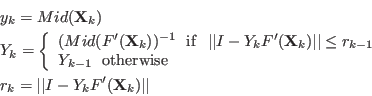
If epsilonf=0, epsilon= and  is the largest
width of the intervals in TestDomain, then the number of boxes
that will be considered in the direct mode
is with, in the worst case:
is the largest
width of the intervals in TestDomain, then the number of boxes
that will be considered in the direct mode
is with, in the worst case:
 |
(2.1) |
where
 is the largest integer greater
than
is the largest integer greater
than  . In the direct storage mode the storage space
will be in the worst case:
. In the direct storage mode the storage space
will be in the worst case:
 |
(2.2) |
In the reverse storage mode the storage space is only:
 |
(2.3) |
Note that with the reverse storage mode, storage is not really a
problem. For example if the width of the initial box is
1000 and the accuracy  , then the necessary storage space is
only 44. Thus only the computation time or the conditioning of the
functions may lead to a failure of the algorithm.
If epsilonf is not equal to 0 the size of the
storage cannot be estimated.
, then the necessary storage space is
only 44. Thus only the computation time or the conditioning of the
functions may lead to a failure of the algorithm.
If epsilonf is not equal to 0 the size of the
storage cannot be estimated.
If the procedure has to be used more than once it is possible to speed
up the computation by allocating the storage space before calling the
procedure. Then you may indicate that the storage space has been
allocated beforehand by indicating a negative value for M, the
number of boxes being given by the absolute value of M.
Note also that the bisection process applied only to one
variable may lead to a better estimation of the roots of the system if
the algorithm stops when the accuracy required on the variable is
reached: indeed, compared to the standard algorithm, one (or more) of
the variable may have been individually split before reaching the step
where a full bisection will lead to a solution (see the example in
section 2.4.3.2).
Note also a specific use of ALIAS_RANDG: if this integer is not
set to 0, then every ALIAS_RANDG iteration the algorithm will
put the box having the largest width as current box, except if the
number of boxes remaining to be processed is greater than half the
total number of available boxes.
Accuracy
Two criterion are used to determine if a box
possibly includes a solution of the system:
- the largest width of the components of the box is lower than epsilon and the functions intervals for this box all contain 0
- the largest width of the function
intervals is lower than epsilonf and they contain all 0. You
must be aware that this test is only used if there is no inequality in
the system. In that case it is compulsory to have an epsilon not equal to 0 otherwise the procedure may lead to an
infinite loop.
If we use only the first criteria (i.e. we put epsilonf=0)
the largest width of the solution intervals will be epsilon. A
consequence is that the unknowns should be normalized in order that
all the intervals in the TestDomain have roughly the same
width.
If we use only the second criteria the width of the solution intervals
cannot be determined and the functions should be roughly normalized
(see the example in section 15.1.3 for the importance of the
conditioning).
Distinct solutions
Two solution intervals will be assumed to contain distinct solutions
if the minimal distance between the middle point of all the intervals
is greater than the threshold Dist.
The procedure will return an integer
 : number of solutions
 : the size of the storage is too low (
possible solutions: increase M,
or use the 3B method, or use the reverse storage mode or the single
bisection mode)
: the size of the storage is too low (
possible solutions: increase M,
or use the 3B method, or use the reverse storage mode or the single
bisection mode)
 : m or n is not strictly positive
 : Order is not 0 or 1
 : one of the function in the system has not a type 0, -1
or 1 (i.e. it's not an equation, neither inequality
: one of the function in the system has not a type 0, -1
or 1 (i.e. it's not an equation, neither inequality  or an
inequality
or an
inequality  )
)
 : we are in the optimization mode and more than one
functions are expressions to be optimized (see the Optimization chapter)
: we are in the optimization mode and more than one
functions are expressions to be optimized (see the Optimization chapter)
 : in the mixed bisection mode the number of variables
that will be bisected is larger than the number of unknowns
: in the mixed bisection mode the number of variables
that will be bisected is larger than the number of unknowns
 : one of the value of ALIAS_Delta3B or
ALIAS_Max3B is negative or 0
: one of the value of ALIAS_Delta3B or
ALIAS_Max3B is negative or 0
 : one of the value of ALIAS_SubEq3B is not 0 or 1
 : although ALIAS_SubEq3B has as size the number of
equations none of its components is 1
: although ALIAS_SubEq3B has as size the number of
equations none of its components is 1
 : ALIAS_ND is different from 0 (i.e. we are
dealing with a non-0 dimensional problem, see the corresponding
chapter) and the name of the result file has not been specified
: ALIAS_ND is different from 0 (i.e. we are
dealing with a non-0 dimensional problem, see the corresponding
chapter) and the name of the result file has not been specified
 : the value of the flag Single_Bisection is not
correct
: the value of the flag Single_Bisection is not
correct
 : we use the full bisection mode and the problem has
more than 10 unknowns
: we use the full bisection mode and the problem has
more than 10 unknowns
Debugging
If the algorithm fail some debugging options are provided. The
integer variable
Debug_Level_Solve_General_Interval indicate
which level of debug is used:
- 0: no debug (the default value)
- 1: during the process are printed on the standard output:
the index of the current box, the
total number of boxes and the number of remaining
boxes
together with the current number of solutions
- 2 : same as 1 but the intervals of the current box
are also printed and when it is split
the new boxes are printed together with their
function intervals
Example 1
We will present first a very silly example of system in the three
unknowns
 :
:
Clearly this system has the unique solution (-1,-1,-1).
We choose to define the TestDomain as the interval [-2,0] for
all three unknowns. So we define a function which specify the TestDomain:
VOID SetTestDomain (INTERVAL_VECTOR & x)
{
  Resize (x, 3);
  x(1) = Hull (-2.0,0.0);
  x(2) = Hull (-2.0,0.0);
  x(3) = Hull (-2.0,0.0);
}
The we have to define the IntervalFunction:
INTERVAL_VECTOR IntervalTestFunction (int l1,int l2,INTERVAL_VECTOR & x)
// interval valued functions. The input are intervals for the
//variables and the output is intervals on the functions
//x are the input variables and xx the function intervals
{
INTERVAL_VECTOR xx(3);

if(l1==1)  xx(1)=x(1)*(x(1)+2)+1;
if(l1<=2 && l2>=2)  xx(2)=x(2)*(x(2)+2)+1;
if(l2==3)  xx(3)=x(3)*(x(3)+2)+1;
  return xx;
}
This function returns the interval vector xx which will contain
the value of the function from l1 to l2 for the box
x. Note that the initial functions have been written
in Horner form (or "nested" form) which may lead to a sharper estimation of the
function intervals.
The main program may be written as:
INT main()
{
int Num; //number of solution
INTERVAL_MATRIX SolutionList(1,3);//the list of solutions
INTERVAL_VECTOR TestDomain;//the input intervals for the variable

//We set the value of the variable intervals
SetTestDomain (TestDomain);

//let's solve....
Num=Solve_General_Interval(3,3,IntervalTestFunction,TestDomain,
      MAX_FUNCTION_ORDER,50000,1,0.001,0.0,0.1,SolutionList,1);
//too much intervals have been created, this is a failure
if(Num== -1)cout << "The procedure has failed (too many iterations)"<<endl;
return 0;
}
This main program will stop as soon as one solution has been found. We
set epsilonf to 0 and epsilon to 0.001 which mean that the
maximal width of the interval solution will be lower than 0.001. The
chosen order is the maximum equation ordering. The number of boxes
should not be larger than 50000 and the distance between the
distinct solutions must be greater than 0.1.
Running this program will provide the solution interval [-1.000977,-1]
for all three variables and uses 71 boxes. The result will
have been similar if we have chosen the maximum middle-point equation
ordering.
On the other hand if we have epsilon to 0 and epsilonf to
0.001 the algorithm find the solution interval [-1.00048828125,-1] and
use 78 boxes.
Now let's look at a more complete test program which enable to test
the various options of the procedure.
INT main()
{
int Iterations;//maximal size of the storage
int Dimension,Dimension_Eq; // size of the system
int Num,i,j,order,precision,Stop;
// accuracy of the solution either on the function  or on the variable
double Accuracy,Accuracy_Variable,Diff_Sol;
INTERVAL_MATRIX SolutionList(200,3);//the list of solutions
INTERVAL_VECTOR TestDomain;//the input intervals for the variable
INTERVAL_VECTOR F(3),P(3);

//We set the number of equations and unknowns and the value of the variable intervals
Dimension_Eq=Dimension=3;
SetTestDomain (TestDomain);

cerr << "Number of iteration = "; cin >> Iterations;
cerr << "Accuracy on Function = "; cin >> Accuracy;
cerr << "Accuracy on Variable = "; cin >> Accuracy_Variable;cerr << "Order (0,1)"; cin >>order;
cerr << "Stop at first solutions (0,1,2):";cin>>Stop_First_Sol;
cerr << "Separation between distincts solutions:";cin>> Diff_Sol;

//let's solve....
Num=Solve_General_Interval(Dimension,Dimension_Eq,IntervalTestFunction,TestDomain,order,Iterations,Stop,
      Accuracy_Variable,Accuracy,Diff_Sol,SolutionList,1);
//too much intervals have been created, this is a failure
if(Num== -1){cout<<"Procedure has failed (too many iterations)"<<endl;return -1;}
cout << Num << " solution(s)" << endl;

for(i=1;i<=Num;i++)
  {
    cout << "solution " << i <<endl;
    cout << "x(1)=" << SolutionList(i,1) << endl;
    cout << "x(2)=" << SolutionList(i,2) << endl;
    cout << "x(3)=" << SolutionList(i,3) << endl;
    cout << "Function value at this point" <<endl;
    for(j=1;j<=3;j++)F(j)=SolutionList(i,j);
    cout << IntervalTestFunction(1,Dimension_Eq,F) <<endl;
    cout << "Function value at middle interval" <<endl;
    for(j=1;j<=3;j++)P(j)=Mid(SolutionList(i,j));
    F=IntervalTestFunction(1,Dimension_Eq,P);
    for(j=1;j<=3;j++)cout << Sup(F(j)) << endl;
  }
  return 0;
}
This program is basically similar to the previous one except that it
enable to define interactively the order, M, Stop, epsilon, epsilonf,Dist. Then it print the solution
together with the function interval for the solution interval and the
value of the functions at the middle point of the solution
interval. Let's test the algorithm to find all he solution (Stop=0) with epsilonf=0 and epsilon=0.001. The algorithm
will fail: indeed let's compute the maximal storage that we may need
using the formula (2.1). We end up with the number
 which is indeed a very large number....
But (2.1) is only an upper bound for the storage. For
example if we have used epsilon=0.01 in the previous formula we
will find that M=
which is indeed a very large number....
But (2.1) is only an upper bound for the storage. For
example if we have used epsilon=0.01 in the previous formula we
will find that M= although the algorithm converge
toward [-1,-0.992188] while
using only 5816 boxes.
although the algorithm converge
toward [-1,-0.992188] while
using only 5816 boxes.
Although academic this system shows several properties of interval
analysis.
If we set epsilon=epsilonf=1e-6, which is the standard
setting of ALIAS-Maple, the algorithm will run for a very long time
before finding the solution of the system. Even using the 3B method,
section 2.3.2 and the 2B method (section 2.17) the
computation time, although improved, will still be very large.
Now if we write the system as
the system will be solved with only 8 boxes, with 2 boxes if we use
the 3B method and without any bisection if we use the 2B method. This
shows clearly the importance of writing the equations in the most
compact form.
Example 2
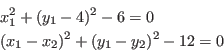
The problem we want to solve is presented in section 15.1.1. We
consider a system of three equations in the unknowns  :
:
which admit the two solutions:
By looking at the geometry of the problem it is easy to establish a
rough TestDomain:
VOID SetTestDomain (INTERVAL_VECTOR & x)
{
  Resize (x, 3);
  x(1) = Hull (0.9,7.1);
  x(2) = Hull (2.1,7.1);
  x(3) = Hull (-Constant::Pi,Constant::Pi);
}
and to determine that the maximum number of real solution is 6.
The IntervalFunction is written as:
INTERVAL_VECTOR IntervalTestFunction (int l1,int l2,INTERVAL_VECTOR & in)
{
INTERVAL_VECTOR xx(3);
if(l1==1)xx(1)=in(1)*in(1)+in(2)*in(2)-50.0;
if(l1<=2 && l2>=2)
  xx(2)=-80.0*Cos(in(3))+90.0+(8.0*Sin(in(3))+in(2))*in(2)+(-20.0+8.0*Cos(in(3))+in(1))*in(1);
if(l2==3)
 xx(3)=92.0-52.0*Cos(in(3))-28.0*Sin(in(3))+(-20.0+4.0*Sin(in(3))+
       4.0*Cos(in(3))+in(2))*in(2)+(-4.0*Sin(in(3))-6.0+4.0*Cos(in(3))+in(1))*in(1);
  return xx;
}
and we may use the same main program as in the previous example
(the name of this program is
Test_Solve_General1).
Let's assume that we set epsilonf to 0 and epsilon to 0.01
while looking at all the solutions (Stop=0), using the maximum equation ordering and
setting Dist to 0.1.
The algorithm provide the following solutions,using 684 boxes:
We notice that indeed none of the roots are contained in the solution
intervals.
If we use the maximum middle-point equation ordering the algorithm
provide the solution intervals, using 684 boxes:
which still does not contain the root (5,5,0) (but contain one of the
root which show the importance of the ordering).
Let's look at what is happening by setting the debug flag
Debug_Level_Solve_General_Interval to 2 (see
section 2.3.4.9).
At some point of the process the algorithm has determined four different
solution intervals:
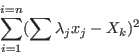
the criteria for the ordering being:
Clearly solution 3 has the lowest criteria and will therefore be stored
as the first solution. Then solution 1 will be considered: but the
distance between the middle point of solution 3 and 1 is lower than
Dist and therefore solution 1 will not be retained. The solution
2 will be considered but for the same reason than for solution 1 this
solution will not been retained. Finally solution 4 will be considered
and it spite of his index being the worse this solution will be
retained as its distance to solution 3 is greater than Dist.
Note that if the single bisection is activated and setting the flag
Single_Bisection to 1 we find the two roots for epsilonf
to 0 and epsilon to 0.01 with 650 boxes using the maximum equation ordering.
We may also illustrate on this example how to deal
with
inequalities. Assume now that we want to deal with the same system but
also with the inequality  . We modify the
IntervalTestFunction as:
. We modify the
IntervalTestFunction as:
INTERVAL_VECTOR IntervalTestFunction (int l1,int l2,INTERVAL_VECTOR & in)
{
INTERVAL x,y,teta;
INTERVAL_VECTOR xx(4);

x=in(1);y=in(2);teta=in(3);
if(l1==1)xx(1)=x*x+y*y-50.0;
if(l1<=2 && l2>=2)
  xx(2)=-80.0*Cos(teta)+90.0+(8.0*Sin(teta)+y)*y+(-20.0+8.0*Cos(teta)+x)*x;
if(l1<=3 && l2>=3)
 xx(3)=92.0-52.0*Cos(teta)-28.0*Sin(teta)+(-20.0+4.0*Sin(teta)+
       4.0*Cos(teta)+y)*y+(-4.0*Sin(teta)-6.0+4.0*Cos(teta)+x)*x;
if(l2==4)
 xx(4)=x*y-22.;
  return xx;
}
Part of the main program will be:
Type(1)=0;Type(2)=0;Type(3)=0;Type(4)=-1;
Num=Solve_General_Interval(3,4,Type,IntervalTestFunction,TestDomain,order,
	Iterations,Stop_First_Sol,Accuracy_Variable,
	Accuracy,Diff_Sol,SolutionList,6);
Here Type(4)=-1; indicates that the fourth function is an
inequality of the type . If we have to deal with the
constraint  then we will use Type(4)=1;.
Example 3
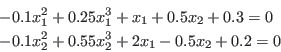
This example is derived from example 2. We notice that in the three
functions of example 2 the second degree terms of  are for all
functions
are for all
functions  . Thus by subtracting the first function to
the second and third we get a linear system in . This system is
solved and the value of are substituted in the first
function. We get thus a system of one equation in the unknown
. Thus by subtracting the first function to
the second and third we get a linear system in . This system is
solved and the value of are substituted in the first
function. We get thus a system of one equation in the unknown
 (see section 15.1.2).
The roots of this equation are 0,-0.806783438.
The test program is Test_Solve_General2.
The IntervalFunction is written as:
(see section 15.1.2).
The roots of this equation are 0,-0.806783438.
The test program is Test_Solve_General2.
The IntervalFunction is written as:
INTERVAL_VECTOR IntervalTestFunction (int l1,int l2,INTERVAL_VECTOR & in)
{
INTERVAL_VECTOR xx(1);
xx(1)=11092.0+(-25912.0+(19660.0-4840.0*Cos(in(1)))*Cos(in(1)))*Cos(in(1))+(
-508.0+(3788.0-1600.0*Cos(in(1)))*Cos(in(1)))*Sin(in(1));
return xx;
}
This program is implemented under the name
Test_Solve_General2.
With epsilonf=0 and epsilon=0.001
we get the solution
intervals, using 32 boxes:
for whatever order.
If we use epsilon=0 and epsilonf=0.1 we get,
using 50 boxes:
In both cases the solution intervals contain the roots of the
equation.
Example 4
In this example (see section 15.1.3) we deal with a complex problem
of three equations in three unknowns
 .
We are looking for a solution in the domain:
.
We are looking for a solution in the domain:
The system has a solution which is approximately:
This problem is extremely ill conditioned as for the TestDomain
the functions intervals are:
This program is implemented under the name Test_Solve_General.
With espsilonf=0 and epsilon=0.001 and if we stop at the
first solution we find with the maximum equation ordering:
with 531 boxes. We may also mention the following
remarks:
- we get no improvement with
the single bisection mode as we need 2435 boxes to find the
first solution,
- using the Reverse Storage mode does not lead to any improvement
for finding the first root: in this mode we need 5587 boxes
to get the first solution,
With the maximum middle-point equation ordering we find:
with 203 boxes.
The importance of normalizing the functions appears if we use epsilonf=0.1 and epsilon=0. If we stop at the first solution we
find:
while if we divide the first function by 1000 we find:
in four time less computation time.
The advantages of the proposed algorithm is that it is easy to use and
implement for a fast check. For sharp system it may provide quickly
solutions with a reasonable accuracy. The drawback is
that it may provide solutions intervals which does not
contain roots or, worse, miss some roots if Dist is not set to 0
(see section 2.3.5.2).
This algorithm may be used also for analysis: if we have to solve
numerous systems we may use this algorithm with a low M in order
to fast check if the current system may have some real roots, in which
case we may consider using a more sophisticated algorithm.
General purpose solving algorithm with Jacobian
Assume now that we are able to compute the jacobian matrix of the
system of functions.
We will use this jacobian for improving the evaluation of the function
intervals using two approaches:
- use the monotonicity of the function
- use the gradient for the evaluation of the function intervals
Note also that this method may be used to solve
a system
composed of equations
,
inequalities
and
inequalities
.
Note also that not all the function must be differentiable to use this
procedure: only one of them is sufficient. In that case you will have
however to set special values in the gradient function
(see 2.4.2.2).
A notable difference with the previous procedure is that we use Moore
theorem (see section 3.1.1) to determine if a unique solution
exists in a given box, in which case we use Krawczyk method for
determining this solution (see section 2.10). Therefore if the
algorithm proposes as solution a point instead of a range this imply
that this solution has been obtained as the result of Moore theorem.
Note however that getting a range for a solution instead of a point
does not always imply that we have a singular solution. For example it
may happen that the solution is exactly at one extremity of a box
(see example in section 2.4.3.2) which a case that our algorithm
does not handle very well. A local analysis of the solution should
however confirm quickly if the solution is indeed singular.
In addition we use also the inflation method presented in
section 3.1.6 to increase the width of the box in which we
may guarantee that there is a unique solution.
Hence this algorithm allows to determine exact solutions in the
sense that we determine boxes that contains a unique solution and
provides a guaranteed numerical scheme that allows for the calculation of the
solution.
In the same way we use the Hansen-Sengupta version of the interval
Newton method to improve the boxes
(see [21]). Note that an improved interval Newton that
may benefit from the structure of the system is
available (see section 3.1.4).
This algorithms allows also to determines the solutions of non-0
dimensional system, see section 2.2.
Using the monotonicity
For a given box we will compute the jacobian matrix using
interval analysis. Each row of this interval matrix enable to get some
information of the corresponding function  .
.
- if the i-th column of the j-th row is an interval which is
strictly negative or strictly positive, then is monotonic with
respect to the unknowns
- if the i-th column of the j-th row is equal to 0, then function
does not depend on the variable
In the first case the minimal and maximal value of will be
obtained either for
 or
or
 and we are able to define the value of to get
successively the minimal and maximal value as we know the sign of the
gradient. But this procedure has to be implemented recursively. Indeed
we have previously computed the jacobian matrix for
and we are able to define the value of to get
successively the minimal and maximal value as we know the sign of the
gradient. But this procedure has to be implemented recursively. Indeed
we have previously computed the jacobian matrix for
 but now
have a fixed value: hence a component
but now
have a fixed value: hence a component  of the j-th row which
for
was such that
of the j-th row which
for
was such that
 and
and
 may now be a strictly positive or negative
intervals. Consequently the minimal and maximal value will be obtained
for some combination of
may now be a strictly positive or negative
intervals. Consequently the minimal and maximal value will be obtained
for some combination of  in the two sets
 and
and
 . Bus as
  has now a fixed value
some other component of
has now a fixed value
some other component of  may become strictly negative or
positive...
may become strictly negative or
positive...
The algorithm for computing a sharper evaluation of is:
 =Evaluate(
)
=Evaluate(
)
- compute
- let
 be the number of components of
  such that
 or
or
 and let
 be the variables for which this occur
- if

loop:
for all combination of
in the set
 :
:
- if

- compute
- let
 be the number of components of such that
or
be the number of components of such that
or
- if
 , then
 =Evaluate(
 )
)
- otherwise
 )
)
- if this is the first estimation of then

- otherwise
- otherwise
-
)
- if this is the first estimation of then
- otherwise
- end loop:
- otherwise
- return
This procedure has to be repeated for each .
Let  be the middle point of
 and
and
 be the box. Then:
 |
(2.4) |
see [5], pp. 52. This expression enable to get in some
cases a sharper bound on .
This evaluation is embedded into the evaluation procedure of the
solving algorithms using the Jacobian. It is also available in its
general form as
INTERVAL_VECTOR Centered_Form(int DimVar,int DimEq,
          INTERVAL_VECTOR (* TheIntervalFunction)(int,int,INTERVAL_VECTOR &),
          INTERVAL_MATRIX (* Gradient)(int, int, INTERVAL_VECTOR &),
          VECTOR &Center,
          INTERVAL_VECTOR &Input)
where
- DimVar: number of variables
- DimEq: number of expressions
- TheIntervalFunction: procedure in MakeF format for
interval evaluating the expressions
- Gradient: procedure in MakeJ format for evaluating
the derivatives of the expressions
- Center:the center point for the centered form
- Input: the ranges for the variables
A variant of this procedure is
INTERVAL Centered_Form(int k,int DimVar,int DimEq,
          INTERVAL_VECTOR (* TheIntervalFunction)(int,int,INTERVAL_VECTOR &),
          INTERVAL_MATRIX (* Gradient)(int, int, INTERVAL_VECTOR &),
          VECTOR &Center,
          INTERVAL_VECTOR &Input)
which is used to evaluate only expression number .
A more sophisticated evaluation for the centered form is based on
Baumann theorem [18]. First we define the procedure
cut(double x,INTERVAL X) as:
For a system of equations in unknowns we define
For a given equation  we use the centered form with as center
with in .
The choice for  is based on the property that the lower
end-point of the centered form
is based on the property that the lower
end-point of the centered form  has a maximum at while
its upper end-point has a minimum at
has a maximum at while
its upper end-point has a minimum at  . The interval evaluation of
 is obtained as
 . Although
  centered form are used to compute the interval evaluation of the
equations the calculation is in fact not so expensive as the interval
evaluation of the Jacobian matrix has to be done only once.
centered form are used to compute the interval evaluation of the
equations the calculation is in fact not so expensive as the interval
evaluation of the Jacobian matrix has to be done only once.
The implementation is:
INTERVAL_VECTOR BiCentered_Form(int DimVar,
          int DimEq,
          INTERVAL_VECTOR (* TheIntervalFunction)(int,int,INTERVAL_VECTOR &),
          INTERVAL_MATRIX (* Gradient)(int, int, INTERVAL_VECTOR &),
          INTERVAL_VECTOR &Input,
          int Exact)
where
- DimVar: number of variables
- DimEq: number of expressions
- TheIntervalFunction: procedure in MakeF format for
interval evaluating the expressions
- Gradient: procedure in MakeJ format for evaluating
the derivatives of the expressions
- Input: the ranges for the variables
- Exact: if 0 the procedure will return as soon as an
interval evaluation of one expression does not include 0
A variant for evaluating only equation number is
INTERVAL_VECTOR BiCentered_Form(int k,int DimVar,
          int DimEq,
          INTERVAL_VECTOR (* TheIntervalFunction)(int,int,INTERVAL_VECTOR &),
          INTERVAL_MATRIX (* Gradient)(int, int, INTERVAL_VECTOR &),
          INTERVAL_VECTOR &Input,
          int Exact)
Another variant is based on the property that the numerical interval
evaluation of the product J(Input)(Input-Center) may be
overestimated as there may be several occurence of the same variable
in this product. We may assume that this product has been computed
symbolically, then re-arranged to reduce the number of occurence of the
same variable leading to a procedure in MakeF format that
computes directly the product. The syntax of the bicentered form
procedure is
INTERVAL_VECTOR BiCentered_Form(int DimVar,
          int DimEq,
          INTERVAL_VECTOR (* TheIntervalFunction)(int,int,INTERVAL_VECTOR &),
          INTERVAL_MATRIX (* Gradient)(int, int, INTERVAL_VECTOR &),
          INTERVAL_VECTOR (* ProdGradient)(int, int, INTERVAL_VECTOR &),
          INTERVAL_VECTOR &Input,
          int Exact)
where ProdGradient is the procedure that computes the product
J(Input)(Input-Center), being understood that the Center
is available in the global variable
ALIAS_Center_CenteredForm.
Single bisection mode
We may use the single bisection mode i.e. bisect only one variable at
a time. Fives modes exist for determining the variable to be bisected,
the choice being made by setting Single_Bisection to a value
from 1 to 8
- 1 : we just split the variable having
the largest width
- 2 : this mode is based on the smear function
as defined by
Kearfott [7]: let
 be the Jacobian
matrix of the system and let define for the variable
the
smear value
be the Jacobian
matrix of the system and let define for the variable
the
smear value
![$s_i = {\rm Max}(
\vert\underline{J_{ij}[\underline{x_i},\overline{x_i}]}\vert,
\vert\overline{J_{ij}[\underline{x_i},\overline{x_i}]}\vert$](img240.png)
![$\forall j\in
[1,n]$](img241.png) where is the total number of functions. The variable that
will be bisected will be the one having the largest
where is the total number of functions. The variable that
will be bisected will be the one having the largest  .
There is however a drawback f the smear function: let consider for
example the equation
.
There is however a drawback f the smear function: let consider for
example the equation  where
where  are large identical
intervals centered at 0.
The derivative of with respect to is
are large identical
intervals centered at 0.
The derivative of with respect to is  and
with respect to
and
with respect to 
 : multiplied by the width of the interval
we get
: multiplied by the width of the interval
we get  and
and  . Hence the smear function for will
be in general larger than for and will always be bisected until its
width is lower than the desired accuracy. Another example in which the
smear function is not the best choice is presented in
section 2.4.3.4.
However the smear function is very often the most efficient mode and
should be privileged.
. Hence the smear function for will
be in general larger than for and will always be bisected until its
width is lower than the desired accuracy. Another example in which the
smear function is not the best choice is presented in
section 2.4.3.4.
However the smear function is very often the most efficient mode and
should be privileged.
- 3 : this is similar to the smear function except that we take
into account its drawback. To avoid bisecting over and over the same
variable we impose that a variable may be considered for bisection
only if the ratio of its width over the maximal width of the box
is not lower than the variable ALIAS_Bound_Smear
(default value 1.e-5).
- 4 : this mode is based on the Krawczyk operator:
to determine which variable should be bisected we
consider the box
![$P=\{[\underline{x_1},\overline{x_1}],\ldots,
[\underline{x_n},\overline{x_n}]\}$](img250.png) . When dealing with the variable
the single bisection mode will lead to two new boxes
. Let
. When dealing with the variable
the single bisection mode will lead to two new boxes
. Let  be the middle point of these boxes
We have seen (section 2.10) that a fundamental point
of Moore test
for determining the unicity of a solution in a box is
that
be the middle point of these boxes
We have seen (section 2.10) that a fundamental point
of Moore test
for determining the unicity of a solution in a box is
that
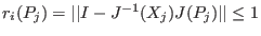 . Thus we will consider in turn
each of the variable and compute the value of
. Thus we will consider in turn
each of the variable and compute the value of  for both . The bisected variable will be chosen as the one leading to the
minimal value of all . However to avoid bisecting over and over
the same variable we use another test: let be the width of the
interval
and be the
maximum of all the . If
we don't consider the
variable as a possible bisection direction.
for both . The bisected variable will be chosen as the one leading to the
minimal value of all . However to avoid bisecting over and over
the same variable we use another test: let be the width of the
interval
and be the
maximum of all the . If
we don't consider the
variable as a possible bisection direction.
- 5: we use a round-robin mode i.e. each variable is
bisected in turn (first , then and so on) unless the width
of the range for the variable is less than the desired accuracy on the
variable, in which case the bisected variable is the next one having a
sufficient width
- 6: like mode 2 of SolveGeneral. ALIAS_RANDG may
still be used to switch between mode 1 and mode 2 of SolveGeneral
- 7: like mode 2 of SolveGeneral except that it is assumed
that the user has defined a simplification procedure that may allow to
reduce the box directly within the bisection process
- 8: the variable are regrouped by groups of
ALIAS_Tranche_Bisection elements. The bisection will look at
each group in turn and bisect the first group that has elements whose
diameter is larger than ALIAS_Size_Tranche_Bisection. When
the element of the group have all elements whose diameter is lower
than this threshold the bisection will consider the next group. If all
elements of all groups have a diameter lower than the threshold the
smear function will be used to determine which variable will be
bisected.
The smear mode leads in general to better result
than the other modes (but there are exception, see example in
section 2.4.3.4).
There is another mode called the mixed bisection: among the
variables we will bisect variables, which will lead to
new boxes. This mode is obtained by setting
the global integer variable
ALIAS_Mixed_Bisection
to  . Here we will order the variables according to the value of
their smear function (if the flag Single_Bisection is 2 or 3) or according to their width (for 1,4,5).
. Here we will order the variables according to the value of
their smear function (if the flag Single_Bisection is 2 or 3) or according to their width (for 1,4,5).
The algorithm is implemented in generic form as:
int Solve_General_Gradient_Interval(int m,int n,
	  INTEGER_VECTOR Type_Eq,
          INTERVAL_VECTOR (* IntervalFunction)(int,int,INTERVAL_VECTOR &),
          INTERVAL_MATRIX (* IntervalGradient)(int, int, INTERVAL_VECTOR &),
          INTERVAL_VECTOR & TheDomain,
          int Order,int M,int Stop,
          double epsilon,double epsilonf,double Dist,
          INTERVAL_MATRIX & Solution,int Nb,INTEGER_MATRIX &GI,
          int (* Simp_Proc)(INTERVAL_VECTOR &))
the arguments being:
- m: number of unknowns
- n: number of functions, see the note 2.3.4.1
- Type_Eq: type of the functions, see the note 2.3.4.2
- IntervalFunction: a function which return the interval
vector evaluation of the functions, see the
note 2.3.4.3. Remember that if you have equations and
inequalities in the system you must first define the equations and
then the inequalities.
- IntervalGradient: a function which the interval matrix of the
jacobian of the functions, see the note 2.4.2.2
- TheDomain: box in which we are looking for
solution of the system. A copy of the search domain is available in
the global variable ALIAS_Init_Domain
- Order: the type of order which is used to store the
boxes created during the bisection process. This order may be
either MAX_FUNCTION_ORDER or MAX_MIDDLE_FUNCTION_ORDER. See the note on the order 2.3.4.4.
- M: the maximum number of boxes which may be
stored. See the note 2.3.4.5
- Stop: the possible values are 0,1,2
- 0: the algorithm will look for every solution in TheDomain
- 1: the algorithm will stop as soon as 1 solution has
been found
- 2: the algorithm will stop as soon as Nb solutions
have been found
- epsilon: the maximal width of the box, see the
note 2.3.4.6
- epsilonf: the maximal width of the function intervals, see the
note 2.3.4.6. Note that if this value is set to 0, then Moore test
is not used.
- Dist: minimal distance between the middle point of two
interval solutions, see the note 2.3.4.7
- Solution: an interval matrix of size (Nb,m)
which will contained the solution intervals. This list is sorted using
the order specified by Order
- Nb: the maximal number of solution which will be returned
by the algorithm
- GI: an integer matrix called the simplified
jacobian, which give a-priori information on
the sign of the derivative of the function. GI(i,j) indicates
the sign of the derivative of function i with respect to
variable j using the following code:
- -1: the derivative is always negative
- 0: the function is not dependent of variable j
- 1: the derivative is always positive
- 2: the sign of the derivative is not known
- Simp_Proc: a user-supplied procedure that take as input
the current box and proceed to some further reduction of
the width of the box components or even determine that there is no
solution for this box, in which case it should return
-1 (see note 2.3.3).
Remember that you may use the 3B method to improve the efficiency of
this algorithm (see section 2.3.2).
Note that the following arguments may be omitted:
- Type_Eq: in that case all the functions will supposed to be
equations.
- GI: in that case all the sign of the derivatives will
supposed to be unknown
- Simp_Proc: no simplification procedure is provided by the
user
The procedure will return an integer
- : number of solutions
- : the size of the storage is too low (
possible solutions: increase M,
or use the 3B method, or use the reverse storage mode or the single
bisection mode)
- : m or n is not strictly positive
- : Order is not 0 or 1
- : one of the function in the system has not a type 0, -1
or 1 (i.e. it's not an equation, an inequality or an
inequality )
- : we are in the optimization mode and more than one
functions are expressions to be optimized (see the Optimization chapter)
- : in the mixed bisection mode the number of variables
that will be bisected is larger than the number of unknowns
- : one of the value of ALIAS_Delta3B or
ALIAS_Max3B is negative or 0
- : one of the value of ALIAS_SubEq3B is not 0 or 1
- : although ALIAS_SubEq3B has as size the number of
equations none of its components is 1
- : ALIAS_ND is different from 0 (i.e. we are
dealing with a non-0 dimensional problem, see the corresponding
chapter) and the name of the result file has not been specified
- : the value of the flag Single_Bisection is not
correct
- : we use the full bisection mode and the problem has
more than 10 unknowns
The following variables play also a role in the computation:
- ALIAS_Store_Gradient: if not 0 the gradient matrix of
each box will be stored together with the input
intervals. Must be set to 0 for large problem
(default value: 1)
- ALIAS_Diam_Max_Gradient: if the maximal width of the
ranges in a box is lower than this value, then the
gradient will be used to perform the interval evaluation of the
functions (default value: 1.e10)
- ALIAS_Diam_Max_Kraw: if the maximal width of the
ranges in a box is lower than this value, then the
Krawczyk operator will be used to determine if there is a unique
solution in the box (default value: 1.e10)
- ALIAS_Diam_Max_Newton: if the maximal width of the
ranges in a box is lower than this value, then the
interval Newton method will be used either to try to reduce
the width of the box or to to ensure that there is no solution of the
system in the box (default value: 1.e10)
Jacobian matrix
The user must provide a function which will compute the interval
evaluation of the jacobian matrix
of its particular functions for a given box. As for the function
evaluation procedure we have chosen a syntax which shows the best
compromise between program calls and interval calculation.
The syntax of this function is:
INTERVAL_MATRIX IntervalGradient (int l1,int l2,INTERVAL_VECTOR & x)
- x: a dimensional interval vector which define the
intervals for the unknowns
- l1,l2: the function must be able to return the interval
evaluation of the component of the jacobian matrix
at row l1 and column l2 i.e. the derivative of the
function number l1 with respect to the variable number l2.
The first row has
number 1, the last n and the first column has number 1, the last
m.
This procedure returns an interval matrix grad of size
m X n in which grad(l1,l2) has been computed.
This function should be written using the BIAS/Profil rules.
Note that if ALIAS_Store_Gradient has not been set to 0 we
will store the simplified Jacobian matrix
for each
box. Indeed if for a given
box B the interval evaluation of one element of the gradient has a
constant sign (indicating a monotonic behavior of the function)
setting the simplified jacobian matrix element to -1 or 1 allows to avoid
unnecessary evaluation of the element of
the Jacobian for the box resulting from a bisection of B as they will
exhibit the same monotonic behavior. Although this idea may sound
quite simple it has a very positive effect on the computation
time. The name of the storage variable of the simplified jacobian is:
INTEGER_MATRIX Gradient_Solve_General_Interval
If a function  is not differentiable you just set the value
of grad(i,..) to the interval [-1e30,1e30]. It is important to
define here a large
interval as the program Compute_Interval_Function_Gradient
that computes the interval evaluation of the function by using their
derivatives uses also the Taylor evaluation based on the value of the
derivatives: a small interval value of the derivatives may lead to a
wrong function evaluation.
is not differentiable you just set the value
of grad(i,..) to the interval [-1e30,1e30]. It is important to
define here a large
interval as the program Compute_Interval_Function_Gradient
that computes the interval evaluation of the function by using their
derivatives uses also the Taylor evaluation based on the value of the
derivatives: a small interval value of the derivatives may lead to a
wrong function evaluation.
Note also that a convenient way to write the Gradient
procedure is to use the procedure MakeJ offered by ALIAS-Maple
(see the ALIAS-Maple manual).
Take care also of the interval valuation
problems of
the element of the Jacobian (see section 2.1.1.3) which may
be different from the one of the functions: for example if a
function is
 it is interval-valuable as soon as the
lower bound of is greater or equal to 0 although the gradient will
involve
it is interval-valuable as soon as the
lower bound of is greater or equal to 0 although the gradient will
involve  which is not interval-valuable if the lower bound of
is equal to 0. ALIAS-Maple offers also the possibility to treat
automatically the interval-valuation problems of the jacobian elements.
which is not interval-valuable if the lower bound of
is equal to 0. ALIAS-Maple offers also the possibility to treat
automatically the interval-valuation problems of the jacobian elements.
Evaluation procedure using the Jacobian
A better evaluation of the function intervals than the IntervalFunction
can be obtained using the Jacobian matrix. A specific procedure
can be used to obtain this evaluation:
INTERVAL_VECTOR Compute_Interval_Function_Gradient(int m,int n,
        INTEGER_VECTOR &Type_Eq,
        INTERVAL_VECTOR (* IntervalFunction)(int,int,INTERVAL_VECTOR &),
        INTERVAL_MATRIX (* IntervalGradient)(int, int, INTERVAL_VECTOR &),
        INTERVAL_VECTOR & Input, int Exact,
        INTEGER_VECTOR &AG,INTEGER_MATRIX &AR)
This procedure computes the function intervals for the box
Input.
- Type_Eq is an integer array whose Dimension_Eq elements
indicates the nature of the functions: -1 for inequality
 , 0 for
equation, 1 for inequality
, 0 for
equation, 1 for inequality  , -2 for a function to be minimized, 2
for a function to be maximized and 10 for a function to be both
minimized and maximized (note that for an optimization problem the
function that has to be minimized must be the last function in the
list of function).
, -2 for a function to be minimized, 2
for a function to be maximized and 10 for a function to be both
minimized and maximized (note that for an optimization problem the
function that has to be minimized must be the last function in the
list of function).
- the integer Exact should be put to 1 as for a value
of 0 the procedure stop the evaluation of each box as soon
as the lower bound of the interval is negative and the upper bound
positive.
- AG is an integer vector of size m x n which
indicates if the sign of some derivatives are already known (the
elements should then have the values -1, 0 or 1) or not (the value
must then be 2)
- AR is a return matrix with the sign of the derivatives for
Input
The parameters Type_Eq, AG, AR may be omitted.
This procedure uses the derivatives for improving the interval
evaluation of the functions in two different ways:
- by taking into account of the monotonicity of the functions
- by using an interval evaluation of the functions based on their
Taylor expansion: it is therefore necessary to evaluate rightly the
derivatives of the functions
The best evaluation of the l-th equation may be computed with
INTERVAL Compute_Interval_Function_Gradient_Line(int l,int Dim_Var,
int Dimension_Eq,
INTERVAL_VECTOR (* IntervalFunction)(int,int,INTERVAL_VECTOR &),
INTERVAL_MATRIX (* Gradient)(int, int, INTERVAL_VECTOR &),
INTERVAL_VECTOR &Input,int Exact,INTEGER_VECTOR &AG)
Storage
The boxes generated by the bisection process are stored in
an interval matrix:
Box_Solve_General_Interval(M,m)
while the corresponding simplified Jacobian matrix is stored in the integer
matrix of size (M, m  n):
n):
Gradient_Solve_General_Interval
called the simplified jacobian: the entry  of this matrix
indicates for function and variable that
the gradient is always positive (1), the gradient is always
negative (-1), the function does not depend upon the variable (0), the
gradient may have not a constant sign within the range of the variable
(2).
The purpose of storing the simplified gradient for each box
is to avoid to re-compute a gradient as soon as it has been
determined that a father of the box has already a gradient
with a constant sign. This has the drawback that for large problems
this storage will be also large: hence it is possible to avoid this
storage by setting the variable
ALIAS_Store_Gradient
to 0 (its default value is 1).
of this matrix
indicates for function and variable that
the gradient is always positive (1), the gradient is always
negative (-1), the function does not depend upon the variable (0), the
gradient may have not a constant sign within the range of the variable
(2).
The purpose of storing the simplified gradient for each box
is to avoid to re-compute a gradient as soon as it has been
determined that a father of the box has already a gradient
with a constant sign. This has the drawback that for large problems
this storage will be also large: hence it is possible to avoid this
storage by setting the variable
ALIAS_Store_Gradient
to 0 (its default value is 1).
The algorithm try to manage the storage in order to solve the problem
with the given number M.
As seen in
section 2.3.1.2 two storage modes are available, the
Direct Storage and the Reverse Storage modes, which
are
obtained by setting the global variable Reverse_Storage to 0
(the default value) or 1.
For both modes
the algorithm will first run until the bisection of the
current box leads to a total number of boxes
which exceed the allowed total number.
It will then delete the boxes
in the list which have been already bisected, thereby freeing some
storage space
(usually larger for the reverse mode than for the direct
mode)
and will start again.
Example 1
This problem has been presented in section 2.3.5.1.
The IntervalGradient function is defined as:
INTERVAL_MATRIX IntervalGradient (int l1,int l2,INTERVAL_VECTOR & x)
{
INTERVAL_MATRIX Grad(3,3);
if(l1==1)
      {
      if(l2==1){Grad(1,1)=2*x(1)+2;return Grad;}
      if(l2==2){Grad(1,2)=0;return Grad;}
      if(l2==3){Grad(1,3)=0;return Grad;}
      }
if(l1==2)
      {
      if(l2==1){Grad(2,1)=0;return Grad;}
      if(l2==2){Grad(2,2)=2*x(2)+2;return Grad;}
      if(l2==3){Grad(2,3)=0;return Grad;}
      }
if(l1==3)
      {
      if(l2==1){Grad(3,1)=0;return Grad;}
      if(l2==2){Grad(3,2)=0;return Grad;}
      if(l2==3){Grad(3,3)=2*x(3)+2;return Grad;}
      }
}
A test main program may now be written as:
INT main()
{
int Num,i,j,order,precision,Stop;
// accuracy of the solution either on the function  or on the variable
double Accuracy,Accuracy_Variable,Diff_Sol;
INTERVAL_MATRIX SolutionList(200,3);//the list of solutions
INTERVAL_VECTOR TestDomain;//the input intervals for the variable
INTERVAL_VECTOR F(3);

//We set the value of the variable intervals
SetTestDomain (TestDomain);

cerr << "Accuracy on Function = "; cin >> Accuracy;
cerr << "Accuracy on Variable = "; cin >> Accuracy_Variable;
cerr << "Order (0,1)"; cin >>order;
cerr << "Stop at first solutions (0,1,2):";cin>>Stop_First_Sol;
cerr << "Separation between distincts solutions:";cin>> Diff_Sol;

//let's solve....
Num=Solve_General_Gradient_Interval(3,3,IntervalTestFunction,
        IntervalGradient,TestDomain,order,10000,Stop,
      Accuracy_Variable,Accuracy,Diff_Sol,SolutionList,1);

//too much intervals have been created, this is a failure
if(Num== -1)cout<<"Procedure has failed (too many iterations)"<<endl;

//otherwise print the solution intervals
for(i=1;i<=Num;i++)
  {
    cout << "solution " << i <<endl;
    cout << "x(1)=" << SolutionList(i,1) << endl;
    cout << "x(2)=" << SolutionList(i,2) << endl;
    cout << "x(3)=" << SolutionList(i,3) << endl;
    cout << "Function value at this point" <<endl;
    for(j=1;j<=3;j++)F(j)=SolutionList(i,j);
    cout << Compute_Interval_Function_Gradient(Dimension,Dimension_Eq,
				     IntervalTestFunction,
				     IntervalGradient,
				     F,1) << endl;
  }
  return 0;
}
A property of this problem is that the Jacobian of the system is
singular at the solution. Hence the unicity test cannot be verified as
it needs to evaluate the inverse of the jacobian matrix (as will fail
the classical Newton scheme, see section 2.9, that needs also
the inverse Jacobian). But even with
epsilon=epsilonf=1e-6 the algorithm is able to find an
approximation of the solution with 16 boxes only. Interestingly this
is a case where the 3B method is not efficient at all: with the 3B
method the number of boxes increases to over 100 000. This is quite
normal: as the 3B method is used before the interval Newton method it
reduces the range for the unknowns toward a region where the interval
Newton method will fail as the Jacobian is close to a singularity. We
therefore end up with a solving that is only based on the bisection
process and we have seen that this process behaves poorly for this
system. But if we mix the 3B method and the 2B filtering of
section 2.17 then the solving needs only 1 box.
Example 2
The problem we want to solve has been presented in
section 2.3.5.2,15.1.1.
The IntervalGradient procedure is:
INTERVAL_MATRIX IntervalGradient (int l1,int l2,INTERVAL_VECTOR & in)
{
INTERVAL_MATRIX Grad(3,3);
INTERVAL x,y,teta;
x=in(1);y=in(2);teta=in(3);
if(l1==1)
  {
    if(l2==1){Grad(1,1)=2*x;return Grad;}
    if(l2==2){Grad(1,2)=2*y;return Grad;}
    if(l2==3){Grad(1,3)=0;return Grad;}
  }
if(l1==2)
  {
    if(l2==1){Grad(2,1)=2.0*x-20.0+8.0*Cos(teta);return Grad;}
    if(l2==2){Grad(2,2)=2.0*y+8.0*Sin(teta);return Grad;}
    if(l2==3){Grad(2,3)=-8.0*x*Sin(teta)+80.0*Sin(teta)+8.0*y*Cos(teta);
      return Grad;}
  }
if(l1==3)
  {
    if(l2==1){Grad(3,1)=2.0*x-6.0+4.0*Cos(teta)-4.0*Sin(teta);
      return Grad;}
    if(l2==2){Grad(3,2)=2.0*y-20.0+4.0*Sin(teta)+4.0*Cos(teta);return Grad;}
    if(l2==3){
      Grad(3,3)=52.0*Sin(teta)-28.0*Cos(teta)+(4.0*Cos(teta)-
              4.0*Sin(teta))*y+(-4.0*Sin(teta)-4.0*Cos(teta))*x;
      return Grad;
             }
  }
}
We may use the same main program as in the previous example
(the name of this program is
Test_Solve_General1_Gradient).
Let's assume that we set epsilonf to 0 and epsilon to 0.01
while looking at all the solutions (Stop=0), using the maximum equation ordering and
setting Dist to 0.1.
The algorithm provide the following solutions after using 55 boxes:
We notice that all of the roots are contained in the solution
intervals.
If we use the maximum middle-point equation ordering the algorithm
provide the same solution intervals.
With epsilonf=0.001, epsilon=0
the algorithm still find exactly the root
with 55 boxes and a computation time of
7010ms. Here Moore test may have failed as the
solution in is 0, which correspond exactly to split point in
the bisection process: it may be useful to break the symmetry
in the test domain.
Using the single bisection mode and setting the flag Single_Bisection to 2 enable to reduce the number of boxes
to 33 and the computation time to 3580ms for epsilonf=0.00001.
Note that we may improve the efficiency of the procedure by using
simplification procedures such as the 2B (section 2.17)
and the 3B method. In that case for
epsilonf=1e-6, epsilon=1e-6 the number of boxes will have been
reduced to 7. Note that the solution [5,5,0] is still not guaranteed.
But using a search space of ![$[-\pi,\pi+1]$](img263.png) for allow the
Moore test to guarantee both solutions.
for allow the
Moore test to guarantee both solutions.
Example 3
This example is derived from example 2. We notice that in the three
equations of example 2 the second degree terms of are for all
functions . Thus by subtracting the first function to
the second and third we get a linear system in . This system is
solved and the value of are substituted in the first
function. We get thus a system of one equation in the unknown
(see section 15.1.2).
The roots of this equation are 0,-0.8067834380. The test program is
Test_Solve_Gradient_General2.
The IntervalGradient function is written as:
INTERVAL_MATRIX IntervalGradient (int l1,int l2,INTERVAL_VECTOR & in)
{
INTERVAL_MATRIX Grad(1,1);
Grad(1,1)=-3788.0+(2692.0+(7576.0-4800.0*Cos(in(1)))*Cos(in(1)))*Cos(in(1))+(
25912.0+(-39320.0+14520.0*Cos(in(1)))*Cos(in(1)))*Sin(in(1));
return Grad;
}
epsilonf=0 and epsilon=0.001
we get the solution by using 8 boxes:
for whatever order.
The solution intervals contain the roots of the
equation.
If we use epsilon=0 and epsilonf=0.1 we get by
using 8 boxes:
Here we get a unique solution and a range solution. But we notice that
the solution 0 is exactly the middle point of the test domain: Moore
test will fail as 0 will always be an end-point of the range. If we
break the symmetry of the test domain we will get exactly both solutions.
Example 4
In this example (see section 15.1.3) we deal with a complex problem
of three equations in three unknowns
.
We are looking for a solution in the domain:
The system has a solution which is approximatively:
This problem is extremely ill conditioned as for the TestDomain
the functions intervals are:
The name of the test program is Test_Solve_General_Gradient.
With espsilonf=0 and epsilon=0.001 and if we stop at the
first solution we find with the maximum equation ordering:
with 73 boxes using the direct storage mode (with the reverse
storage mode only 37 boxes are needed).
With the maximum middle-point equation ordering we find the same intervals
with 67 boxes in the direct storage mode (41 for the
reverse storage mode).
The importance of normalizing the functions has been mentioned in
section 2.3.5.4. But in this example the use of the Jacobian matrix
enable to drastically reduce the computation time.
If we use epsilonf=0.1 and epsilon=0 and if we stop at the first solution we
find an exact solution using 73 boxes:
in a time which is about 1/100 of the time necessary when we
don't use
the Jacobian.
In the single bisection smear mode (i.e. only one variable is
bisected in the process) the same root is obtained in 21080ms (about
50% less time than when using the full bisection mode) with
only 40 boxes in the direct storage mode.
Note that for epsilonf=0.1 and epsilon=0 we find the only root with 73
boxes in 39760ms
(41 boxes and 24650ms in the single bisection smear mode).
Note that we may improve the efficiency of the procedure by using
simplification procedures such as the 2B (section 2.17)
and the 3B method. An interesting point in this example is that the
bisection mode 1 (bisecting along the variable whose interval has the
largest diameter) is more effective than using the bisection mode 2
(using the smear function) with 53 boxes against 108 for the mode 2
for epsilonf=1e-6 and epsilon=1e-6.
This can easily been explained by the complexity of the Jacobian
matrix elements that leads to a large overestimation of their values
when using interval: in that case the smear function is not very
efficient to determine which variable has the most influence on the
equations.
According to the system this procedure may not be especially faster
than the general purpose
algorithm but the number of necessary boxes is in general
drastically reduced. Furthermore the use of Moore test and interval
Newton method enable in many
cases to determine exactly the solutions.
General purpose solving algorithm with Jacobian and Hessian
In this new algorithm we will try to improve the evaluation of the
function intervals by using the Hessian of the functions. This
improvement is based on a sharper analysis of the monotonicity of the
functions which in turn is based on a sharper evaluation of the
Jacobian matrix of the system. The element  of the Jacobian matrix
at row and column is:
of the Jacobian matrix
at row and column is:
Now consider the corresponding line of the Hessian matrix which is:
The elements of this line indicate the monotonic behavior of the
elements of the Jacobian matrix. If some elements in this line have a
constant sign, then the elements of the Jacobian are monotonic with
respect to some of the unknowns and using this monotonicity we may
improve the evaluation of the element of the Jacobian
matrix. This improvement has to be
applied recursively: indeed as we will evaluate the Jacobian elements
for boxes in which some components have now a fixed
value the evaluation of the Hessian matrix for these boxes
may lead to a larger number of the component of the Hessian which have
a constant sign. The recursion will stop if all the component of the
Hessian line have a constant sign or if the number of component with a
constant sign does not increase.
Note also that not all the function must be differentiable to use this
procedure: only one of them is sufficient. In that case you will have
however to set special values in the gradient and hessian function
(see 2.4.2.2).
We will also use the Hessian in order to try to sharpen the evaluation
of . Let the box intervals be
 .
Let be the middle point of
and
be the box. Then:
.
Let be the middle point of
and
be the box. Then:
 |
(2.5) |
see [5], pp. 52. This expression enable to get in some
cases a sharper bound on .
The improvement of the evaluation of the function intervals is due to
the fact that a sharper evaluation of the Jacobian matrix may lead to
a larger number of Jacobian elements with constant sign than with the
direct evaluation of the Jacobian matrix. To speed up the algorithm we
store the Jacobian matrix of each box: this enable to
avoid the evaluation of the components of the Jacobian matrix which
have a constant sign when bisecting the box
Another interest of the Hessian is that it enable to use Kantorovitch
theorem. This theorem (see section 3.1.2) can be applied if the
number of unknowns is equal to the number of equations and
enable to determine boxes in which there is an unique
solution, solution which can be found using Newton method (see
section 2.9) with as estimate of the solution any point
within the boxes.
We will use this theorem at three possible levels:
- level 0: we want solution intervals for which the maximal width is equal
or lower than a given threshold. In that case imagine that two
solution intervals have been found at some point of the algorithm,
this two solutions being close. We will apply Kantorovitch theorem for
the center of the two solution intervals. In the most favorable case
one of them will contain an unique solution while the boxes
given by Kantorovitch theorem will cover the other one: consequently
this input intervals will be eliminated of the solution
intervals. Therefore Kantorovitch theorem will eliminate spurious
solution intervals and we don't need to indicate a minimal distance
between the solution intervals.
- level 1: we look for solution intervals whose width has no importance as
soon as we are sure that they contain one unique solution which can be
found using Newton method with as estimate of the solution any point
within the solution intervals. In that case we will apply Kantorovitch
theorem for each boxes which appear during the algorithm. If
the theorem give a solution intervals we will store it in the solution
list and update the remaining boxes of the list so that none
of them contain the solution intervals. A consequence is that the
width of the solution intervals cannot be determined beforehand while
each solution intervals that have been determined using this method
contain one unique solution which can be determined using Newton
method.
- level 2: we apply Newton method for each box and if
Newton converge toward a solution within the current box we
store the box as solution interval. The boxes in the list are then
filtered so that none of them contains the solution interval.
Furthermore we use the inflation method presented in
section 3.1.6 to increase the width of the box in which we
may guarantee that there is a unique solution.
As for the method using only the gradient
we use the Hansen-Sengupta version of the interval
Newton method to improve the
boxes
(see [21]).
Single bisection mode
Instead of bisecting all the variables we may bisect only one of the
variable. The criteria for determining which of the variable will be
bisected is identical to the one presented in section 2.4.1.3
for the mode up to 5. The mode 6 is different: basically we will
bisect the variable having the largest diameter except that it is
supposed that
a weight is assigned to each variable and the diameter used by the
bisection process is the diameter of the range for the variable
multiplied by the weight of the variable. The weight must be indicated
in the vector ALIAS_Bisection_Weight.
The generic implementation of this solving procedure is:
int Solve_General_JH_Interval(int Dimension_Var,int Dimension_Eq,
			      INTEGER_VECTOR &Type_Eq,
	INTERVAL_VECTOR (* TheIntervalFunction)(int,int,INTERVAL_VECTOR &),
		INTERVAL_MATRIX (* Gradient)(int, int,INTERVAL_VECTOR &),
		INTERVAL_MATRIX (* Hessian)(int, int, INTERVAL_VECTOR &),
		INTERVAL_VECTOR & TheDomain,
		int Order,
		int Iteration,
		int Stop_First_Sol,
		double Accuracy_Variable,
		double Accuracy,
		INTERVAL_MATRIX & Solution,
                INTEGER_VECTOR & Is_Kanto,
		int Apply_Kanto,
			      int Nb_Max_Solution,INTERVAL_MATRIX &Grad_Init,
			      int (* Simp_Proc)(INTERVAL_VECTOR &),
			      int (* Local_Newton)(int Dimension,int Dimension_Eq,
	  INTERVAL_VECTOR (* TheIntervalFunction)(int,int,INTERVAL_VECTOR &),
	  INTERVAL_MATRIX (* Gradient)(int, int, INTERVAL_VECTOR &),
	  VECTOR &Input,double Accuracy,int Max_Iter, VECTOR &Residu,INTERVAL_VECTOR &In))
the arguments being:
- m: number of unknowns
- n: number of functions, see the note 2.3.4.1
- Type_Eq: type of the functions, see the note 2.3.4.2
- IntervalFunction: a function which return the interval
vector evaluation of the functions, see the
note 2.3.4.3. Remember that if you have equations and
inequalities in the system you must first define the equations and
then the inequalities.
- IntervalGradient: a function which return
the interval matrix of the
jacobian of the functions, see the note 2.4.2.2
- IntervalHessian: a function which return
the interval matrix of the
Hessian of the functions, see the note 2.5.2.1
- TheDomain: box in which we are looking for
solution of the system. A copy of the search domain is available in
the global variable ALIAS_Init_Domain
- Order: the type of order which is used to store the
intervals created during the bisection process. This order may be
either MAX_FUNCTION_ORDER or MAX_MIDDLE_FUNCTION_ORDER. See the note on the order 2.3.4.4.
- M: the maximum number of
boxes which may be
stored. See the note 2.5.2.2
- Stop: the possible values are 0,1,2
- 0: the algorithm will look for every solution in TheDomain
- 1: the algorithm will stop as soon as 1 solution has
been found
- 2: the algorithm will stop as soon as Nb solutions
have been found
- epsilon: the maximal width of the box, see the
note 2.3.4.6
- epsilonf: the maximal width of the function intervals, see the
note 2.3.4.6
- Solution: an interval matrix of size (Nb,m)
which will contained the solution intervals. Each solution may be:
- a set of intervals with the associated flag IsKanto to 0:
- a set of intervals with the associated flag IsKanto to 1: there is an unique solution in the set and Newton
method will converge toward this solution
- a set of intervals reduced to a point with the
associated flag IsKanto to 0: this point is a solution which has been obtained with Krawczyk
method (see 2.10). The accuracy of this solution may be improved
by using the point as starting point for Krawczyk
method and decreasing the accuracy epsilonf
- IsKanto: an integer vector of dimension Nb. A value
of 1 for IsKanto(i)
indicate that applying Newton method (see section 2.9)
with as estimate the center of the solution intervals Solution(i) will
converge toward the unique solution which lie within the
solution intervals Solution(i)
- ApplyKanto: an integer which indicate at which
level we use Kantorovitch theorem. If 1 we use Kantorovitch theorem
(see section 3.1.2 and the mathematical
background) to determine the solution. A consequence is
that the solution interval may have a width larger than epsilon. If 0 we use Kantorovitch theorem just to separate the
solutions: the solution interval will have a width epsilon.
If 2 we will apply Newton method for every box which has not been
eliminated during the bisection process but we will consider the
result a solution only if it lie within the box. The maximal number of
iteration is determined by the global variable Max_Iter_Newton_JH_Interval (by default
100).
In that case we may miss solutions if they are lying inside the same box.
- Nb: the maximal number of solution which will be returned
by the algorithm
- GM: an interval matrix which give a-priori information on
the values of the derivatives of the function. GM(i,j) is the
interval value of the derivative of function i with respect to
variable j
- Simp_Proc: a user-supplied procedure that take as input
the current box and proceed to some further reduction of
the width of the box or even determine that there is no
solution for this box, in which case it should return
-1 (see note 2.3.3).
Remember that you may use the 3B method to improve the efficiency of
this algorithm (see section 2.3.2).
- Local_Newton: a Newton scheme that is used when Apply_Kanto is set to 2. When omitted the algorithm will use the
ALIAS Newton procedure (see section 2.9).
Note that the following arguments may be omitted:
- Type_Eq: in that case all the functions will supposed to be
equations.
- GM: in that case all the derivatives will
supposed to be unknown
- Simp_Proc: no simplification procedure is provided by the
user
- Local_Newton
The following variables play also a role in the computation:
- ALIAS_Store_Gradient: if not 0 the gradient matrix of
each box will be stored together with the boxes.
Must be set to 0 for large problem
(default value: 1)
- ALIAS_Diam_Max_Gradient: if the maximal width of the
ranges in a box is lower than this value, then the
gradient will be used to perform the interval evaluation of the
functions (default value: 1.e10)
- ALIAS_Diam_Max_Kraw: if the maximal width of the
ranges in a box is lower than this value, then the
Krawczyk operator will be used to determine if there is a unique
solution in the box (default value: 1.e10)
- ALIAS_Diam_Max_Newton: if the maximal width of the
ranges in a box is lower than this value, then the
interval Newton method will be used either to try to reduce
the width of the box or to to ensure that there is no solution of the
system in the box (default value: 1.e10)
- ALIAS_Always_Use_Inflation: if ApplyKanto is set
to 1 we get for each solution a box
 which contains only one
solution. If this flag is set to 1 we compute the solution using
Newton and then we use an inflation procedure that try to determine a
box
which contains only one
solution. If this flag is set to 1 we compute the solution using
Newton and then we use an inflation procedure that try to determine a
box  which is larger than and contains also only one solution
- ALIAS_Eps_Inflation: the inflation algorithm will try to
increase the width of the box by at least this value
- ALIAS_Sing_Determinant: if the determinant of the
jacobian matrix of the system is lower than this value, then the
system is supposed to be singular
- ALIAS_Diam_Sing: for a value
 of this
parameter if there is singular solution in the
system, then the algorithm will not look for solution of the system in
a box of width 2 around the singular solution (default value: 0)
of this
parameter if there is singular solution in the
system, then the algorithm will not look for solution of the system in
a box of width 2 around the singular solution (default value: 0)
- ALIAS_Use_Grad_Equation: if this integer array has a
size of n the derivatives of equation will be used to
evaluate the i-th equation only if ALIAS_Use_Grad_Equation[i]
is not 0
- ALIAS_No_Hessian_Evaluation: if set to 0 we will not
use the Hessian to sharpen the interval evaluation of the Gradient
when performing the interval evaluation of the equations. This may be
useful if its known that the interval evaluation of the elements of
the hessian will
have always a constant sign
Hessian procedure
The syntax of this function is:
Hess=INTERVAL_MATRIX IntervalHessian (int l1,int l2,INTERVAL_VECTOR & in)
This procedure should return an interval matrix of
size m n, m in which the Hessian of function
numbered l1 to l2 has been updated (function number start
at 1). The Hessian matrix of
function (which is of size n m) is stored at
location Hess((-1)m+1 m,1m).
Remember that for each function the Hessian matrix is symmetric: this
fact should be used in order to speed up the evaluation of this
matrix.
If a function in the system is not
m,1m).
Remember that for each function the Hessian matrix is symmetric: this
fact should be used in order to speed up the evaluation of this
matrix.
If a function in the system is not  you set all the elements of
its hessian matrix to the interval [-1e30,1e30]. Remember also here to
verify that each element of the Hessian should be interval-valuable
(see section 2.1.1.3).
you set all the elements of
its hessian matrix to the interval [-1e30,1e30]. Remember also here to
verify that each element of the Hessian should be interval-valuable
(see section 2.1.1.3).
Storage
The boxes generated by the bisection process are stored in
an interval matrix:
Box_Solve_General_Interval(M,m)
while the corresponding Jacobian matrix is stored in the interval
matrix of size (M, m n):
Gradient_Solve_JH_Interval
The purpose of storing the gradient for each box
is to avoid to re-compute a gradient as soon as it has been
determined that a father of the box has already a gradient
with a constant sign. This has the drawback that for large problems
this storage will be also large: hence it is possible to avoid this
storage by setting the variable
ALIAS_Store_Gradient
to 0 (its default value is 1).
Note that here we store the interval gradient matrix and not the
simplified gradient matrix as in the solving procedure
involving only the Jacobian.
The algorithm try to manage the storage in order to solve the problem
with the given number M (see section 2.3.1.2).
As seen in
section 2.3.1.2 two storage modes are available, the
Direct Storage and the Reverse Storage modes, which
are
obtained by setting the global variable Reverse_Storage to 0
(the default value) or to the number of
unknowns+1.
For both modes
the algorithm will first run until the bisection of the
current box leads to a total number of boxes
which exceed the allowed total number.
It will then delete the boxes
in the list which have been already bisected, thereby freeing some
storage space
(usually larger for the reverse mode than for the direct
mode)
and will start again.
If the procedure has to be used more than once it is possible to speed
up the computation by allocating the storage space before calling the
procedure. Then you may indicate that the storage space has been
allocated beforehand by indicating a negative value for M, the
number of boxes being given by the absolute value of M.
An improved value of the Jacobian is obtained by taking account its
derivative in the procedure:
INTERVAL_MATRIX Compute_Best_Gradient_Interval(int Dimension,
                    int Dimension_Eq,
                    INTERVAL_MATRIX (* Gradient)(int, int, INTERVAL_VECTOR &),
                    INTERVAL_MATRIX (* Hessian)(int, int, INTERVAL_VECTOR &),
                    INTERVAL_VECTOR &Input,
                    int Exact,INTERVAL_MATRIX &InGrad)
where
- Exact: if 1 the calculation for one element of the
Jacobian will stop as soon as the
method has found that the interval evaluation of the element will not
have a constant sign. If 0 the best interval evaluation will be
computed
- InGrad: if this matrix is not the zero matrix we will
assume that the non zero elements of this matrix are the interval
evaluation of the Jacobian
To compute only the best value of the jacobian element at l-th row nad
j-th column you may use:
INTERVAL Compute_Best_Gradient_Interval_line(int l,int j,int Dim,
                    int Dimension_Eq,
                    INTERVAL_MATRIX (* Gradient)(int, int, INTERVAL_VECTOR &),
                    INTERVAL_MATRIX (* Hessian)(int, int, INTERVAL_VECTOR &),
                    INTERVAL_VECTOR &Input,int Exact)
We may also obtain the best interval evaluation of the equations
through the procedure
INTERVAL_VECTOR Compute_Interval_Function_Gradient(int Dimension,
                    int Dimension_Eq,
                    INTERVAL_VECTOR (* TheIntervalFunction)(int,int,INTERVAL_VECTOR &),
                    INTERVAL_MATRIX (* Gradient)(int, int, INTERVAL_VECTOR &),
                    INTERVAL_MATRIX (* Hessian)(int, int, INTERVAL_VECTOR &),
                    INTERVAL_VECTOR &Input, int Exact)
The procedure will return an integer
- : number of solutions
- : the size of the storage is too low (
possible solutions: increase M,
or use the 3B method, or use the reverse storage mode or the single
bisection mode)
- : m or n is not strictly positive
- : Order is not 0 or 1
- : one of the function in the system has not a type 0, -1
or 1 (i.e. it's not an equation, neither inequality or an
inequality )
- : in the mixed bisection mode the number of variables
that will be bisected is larger than the number of unknowns
- : one of the value of ALIAS_Delta3B or
ALIAS_Max3B is negative or 0
- : one of the value of ALIAS_SubEq3B is not 0 or 1
- : although ALIAS_SubEq3B has as size the number of
equations none of its components is 1
- : ALIAS_ND is different from 0 (i.e. we are
dealing with a non-0 dimensional problem, see the corresponding
chapter) and the name of the result file has not been specified
- : the value of the flag Single_Bisection is not
correct
- : we use the full bissection mode and the problem has
more than 10 unknowns
As for the debug option they have been presented in the section 2.3.4.9.
Example 2
The problem we want to solve has been presented in
section 2.3.5.2 and section 15.1.1.
The name of the test program is Test_Solve_JH_General1.
If epsilonf=0.01 the program using the maximum equation ordering find
the two solutions using 50 boxes.
If we use the single bisection smear mode the program using the maximum equation ordering find
the two solutions in 4260ms using 32 boxes.
Note that we may improve the efficiency of the procedure by using
simplification procedures such as the 2B (section 2.17)
and the 3B method. In that case for
epsilonf=1e-6, epsilon=1e-6 the number of boxes will have been
reduced to 2 and both solutions will be guaranteed.
even with a search space of ![$[-\pi,\pi]$](img277.png) for .
for .
This example is derived from example 2 and has been presented in
section 2.3.5.3.
The test program is Test_Solve_JH_General2.
The IntervalFunction and IntervalGradient have been presented
before. The IntervalHessian is:
INTERVAL_MATRIX IntervalHessian (int l1,int l2,INTERVAL_VECTOR & in)
{
INTERVAL_MATRIX Hess(1,1);
Hess(1,1)=39320.0+(-3128.0+(-78640.0+43560.0*Cos(in(1)))*
      Cos(in(1)))*Cos(in(1))+(-2692.0+(-15152.0+14400.0*Cos(in(1)))*
      Cos(in(1)))*Sin(in(1));
return Hess;
}
A test main program may be written as:
INT main()
{
int Iterations,Dimension,Dimension_Eq,Apply_Kanto;
int Num,i,j,order,Stop_First_Sol,precision,niter,nn;
double Accuracy,Accuracy_Variable,eps;
INTERVAL_MATRIX SolutionList(200,3);
INTERVAL_VECTOR TestDomain,F(1),P(1),H(3);
VECTOR TR(1),Residu(1);
INTEGER_VECTOR Is_Kanto(6);

Dimension_Eq=Dimension=1;SetTestDomain (TestDomain);

cerr << "Number of iteration = "; cin >> Iterations;
cerr << "Accuracy on Function = "; cin >> Accuracy;
cerr << "Accuracy on Variable = "; cin >> Accuracy_Variable;
cerr << "Debug Level (0,1,2)="; cin >> Debug_Level_Solve_General_Interval;
cerr << "Order (0,1)="; cin >>order;
cerr << "Stop at first solutions (0,1,2)=";cin>>Stop_First_Sol;
cerr << "Apply Kanto (0,1)=";cin>>Apply_Kanto;

Num=Solve_General_JH_Interval(Dimension,Dimension_Eq,
      IntervalTestFunction,IntervalGradient,IntervalHessian,
      TestDomain,order,Iterations,Stop_First_Sol,Accuracy_Variable,
      Accuracy,SolutionList,Is_Kanto,Apply_Kanto,6);

if(Num== -1){cout << "The procedure has failed (too many iterations)"<<endl;return 0;}
cout << Num << " solution(s)" << endl;
for(i=1;i<=Num;i++)
  {
    cout<<"solution "<<i<<endl;cout<<"teta="<<SolutionList(i,1)<<endl;
    cout << "Function value at this point" <<endl;F(1)=SolutionList(i,1);
    cout << Compute_Interval_Function_Gradient(Dimension,Dimension_Eq,
				     IntervalTestFunction,IntervalGradient,
      			     IntervalHessian,F,1) << endl;
    cout << "Function value at middle interval" <<endl;
    P(1)=Mid(SolutionList(i,1));    F=IntervalTestFunction(1,Dimension_Eq,P);
    cout << Sup(F(1)) << endl;    TR(1)=Mid(SolutionList(i,1));
    if(Is_Kanto(i)==1)cout << "This solution is Kanto" <<endl;
    else cout << "This solution is not Kanto" << endl;
    if(Kantorovitch(Dimension,IntervalTestFunction,IntervalGradient,
                             IntervalHessian,TR,&eps)==1)
      {
	P(1)=INTERVAL(TR(1)-eps,TR(1)+eps);
	cout << "Unique solution in: " <<P << endl;
      }
    if(Is_Kanto(i)==1)
      {
      nn=Newton(Dimension,IntervalTestFunction,IntervalGradient,TR,Accuracy,1000,Residu);
      if(nn>0)
        {
          cout << "Newton iteration converge toward: " << endl;
          cout << TR << "with residu= " << Residu<< endl;
        }
      else
        {
          if(nn==0)cout << "Newton does not converge" << endl;
          if(nn== -1)cout<<"Newton has encountered a singular matrix"<<endl;
        }
      }
  }
  return 0;
}
With epsilonf=0.0001 and epsilon=0.001 , using Kantorovitch at
level 1,
we get the solution
intervals, using 4 boxes:
Newton method initialized with the center of these boxes
converge toward 4.08282e-15 and -0.8067834.
In this example (see section 15.1.3) we deal with a complex problem
of three equations in three unknowns
.
We are looking for a solution in the domain:
The system has a solution which is approximatively:
This problem is extremely ill conditioned as for the TestDomain
the equations intervals are:
The name of the test program is Test_Solve_JH_General.
If we use epsilonf=0.1 and epsilon=0, we get the first solution
with the following number of boxes and computation time:
|
|
full bisection |
smear bisection |
|
direct storage |
71, 31200ms |
38, 20220ms |
|
reverse storage |
35, 14710ms |
38, 20280ms |
Note that we may improve the efficiency of the procedure by using
simplification procedures such as the 2B (section 2.17)
and the 3B method. An interesting point in this example is that the
bisection mode 1 (bisecting along the variable whose interval has the
largest diameter) is more effective than using the bisection mode 2
(using the smear function) with 33 boxes against 38 for the mode 2
for epsilonf=1e-6 and epsilon=1e-6.
This can easily been explained by the complexity of the Jacobian
matrix elements that leads to a large overestimation of their values
when using interval: in that case the smear function is not very
efficient to determine which variable has the most influence on the
equations. But it must be noted that the use of the Hessian allows to
reduce this overestimation and consequently the differences in term of
used boxes between the two bisection mode is slightly reduced compared
to the one we have observed when using only the Jacobian (see
section 2.4.3.4).
It may be interesting to stop the solving procedures although the
algorithm has not been completed. We have already seen that a possible
mean to do that was to specify a number of roots in such way that the
procedure will exit as soon it has found this number of roots.
Another possible way to stop the calculation is to use a time-out
mechanism. For that purpose you may define in the
double ALIAS_TimeOut the maximum number of minutes allowed for the
calculation. If this number is reached (approximatively) the procedure
will exit and will set the flag
ALIAS_TimeOut_Activated to 1.
The solution that have been found by the algorithms are stored in the
interval matrix ALIAS_Solution and their number is
ALIAS_Nb_Solution.
Note that for the procedures involving the Jacobian this matrix will
usually describes the boxes that include a unique solution.
Ridder method for solving one equation
Ridder method is an iterative scheme used to obtain one root of the
equation  within an interval
 ![$[x_1,x_2]$](img280.png) . It assumes that
. It assumes that
 . Let
. Let  be the mid-point of the interval
. A new estimate of the root is
be the mid-point of the interval
. A new estimate of the root is  with:
with:
under the assumption
it may be seen that is
guaranteed to lie within the interval . As soon as as
been determined we choose as new the interval ![$[x_1,x_4]$](img285.png) if
if
 or
or ![$[x_4,x_2]$](img287.png) if
if
 . The convergence
of this algorithm is quadratic.
Ridder's method enable to find a root of an equation as soon
as the root is bracketed in an interval such that
. It is implemented as:
. The convergence
of this algorithm is quadratic.
Ridder's method enable to find a root of an equation as soon
as the root is bracketed in an interval such that
. It is implemented as:
int Ridder(REAL (* TheFunction)(REAL),INTERVAL &Input,
      double AccuracyV,double Accuracy,int Max_Iter,double *Sol, double *Residu)
with:
- TheFunction: a procedure which enable to compute the value
of the equation at a given point
- Input: the interval in which we are looking
for a root
- AccuracyF: a threshold on the minimal value of the width of the
interval
![$[x_k, x_{k+1}]$](img289.png) with
with
 considered during the procedure
- Accuracy: a threshold on the value of
 which
determine a root of the equation
which
determine a root of the equation
- MaxIter: maximal number of iteration
- Sol: on success the value of the root
- Residu: the value of the equation at Sol
The procedure returns:
- 1: a solution has been found as F(Sol)
 Accuracy
- 2: a solution has been found as
 AccuracyV
- -1:
- -2: a numerical error was encountered during the computation
- -3: the maximal number of iteration has been reached without
finding a solution
The test program Test_Ridder2 present a program to solve the
trigonometric equation presented as example 2 (see
section 15.1.1).
Brent method for solving one equation
Brent method is an iterative scheme used to obtain one root of the
equation within an interval . It assumes that
. Let be the mid-point of the interval
. A new estimate of the root is with:
with:
In this method is considered to be the current estimate of the
solution. The term  is a correction factor: when this factor
leads to a new estimate of the solution outside the interval we use a
bisection method to compute a new interval . In other words
if
is a correction factor: when this factor
leads to a new estimate of the solution outside the interval we use a
bisection method to compute a new interval . In other words
if
 the new interval is
 ![$[x_1,x_3]$](img299.png) and if
and if
 the new interval is
 ![$[x_3,x_2]$](img301.png) . Therefore Brent
method is a cross between a bisection method and a super-linear method
which insure that the estimate of the solution always lie within the
interval .
. Therefore Brent
method is a cross between a bisection method and a super-linear method
which insure that the estimate of the solution always lie within the
interval .
Brent's method enable to find a root of an equation as soon
as the root is bracketed in an interval such that
. It is implemented as:
int Brent(REAL (* TheFunction)(REAL),INTERVAL &Input,
      double AccuracyV,double Accuracy,int Max_Iter,double *Sol, double *Residu)
with:
- TheFunction: a procedure which enable to compute the value
of the equation at a given point
- Input: the interval in which we are looking
for a root
- AccuracyF: a threshold on the minimal value of the width of the
interval
with
considered during the procedure
- Accuracy: a threshold on the value of which
determine a root of the equation
- MaxIter: maximal number of iteration
- Sol: on success the value of the root
- Residu: the value of the equation at Sol
The procedure returns:
- 1: a solution has been found as F(Sol)Accuracy
- 2: a solution has been found as
AccuracyV
- -1:
- -3: the maximal number of iteration has been reached without
finding a solution
The test program Test_Ridder2 present a program to solve the
trigonometric equation presented as example 2 (see
section 15.1.1).
Newton method for solving systems of equations
Let  be a system of equations in the unknowns
  and
and  be an estimate of the solution of the system.
Let
be an estimate of the solution of the system.
Let  be the Jacobian matrix of the system of equation. Then
the iterative scheme defined by:
be the Jacobian matrix of the system of equation. Then
the iterative scheme defined by:
 |
(2.6) |
starting with may converge toward a solution of the system.
A simplified Newton method consist in using a constant matrix in
the classical Newton method, for example the inverse Jacobian matrix
at some point like . The iterative scheme become:
 |
(2.7) |
Although the simplified method may need a larger number of iteration
before converging than the classical scheme each iteration has a lower
computation time as there is no computation of the
inverse of the Jacobian matrix. This method may also encounter
convergence
problem as it has a
convergence ball smaller than the classical Newton method.
Newton method has advantages and drawbacks that need to be known in
order to use it in the best way:
- it may really be fast: this may be important, for example in
real-time control
- it is very simple to use
- but it does not necessarily converge toward the solution
"closest" to the estimate (see the example in section 15.1.2)
- but it may not converge. Kantorovitch theorem
(see
section 3.1.2) enable to determine the size of the convergence
ball but this size is usually small (but quite often in practice the
size
is greater than the size given by the theorem which however is exact
in some cases)
- but a numerical implementation of Newton may overflow
The procedure for using Newton method is:
int Newton(int n,VECTOR (* TheFunction)(VECTOR &),
        MATRIX (* Gradient)(VECTOR &),
        VECTOR &Input,double Accuracy,int MaxIter,VECTOR &Residu)
with
- n: number of equations
- TheFunction: a procedure which return the value of the
equation for given values of the unknowns (see note 2.3.4.3)
- Gradient: a procedure which return the Jacobian matrix of
the system for given values of the unknowns (see note 2.4.2.2)
- Input: at the start of the procedure the estimate of the
solution, at the end of the procedure the solution
- Accuracy: the procedure return a solution if there is an
Input such that
 for all in [1,].
- MaxIter: the procedure will return a failure code if a
solution is not found after MaxIter iteration
- Residu: the value of the equations for the solution
Note that it also possible to use in the Newton method
the interval evaluation of the
equation and of the Jacobian matrix which are necessary for the
general purpose solving algorithm with Jacobian (see
section 2.4). The syntax of this implementation
is:
int Newton(int Dimension,
        INTERVAL_VECTOR (* IntervalFunction)(int,int,INTERVAL_VECTOR &),
        INTERVAL_MATRIX (* IntervalGradient)(int, int, INTERVAL_VECTOR &),
        VECTOR &Input,double Accuracy,int MaxIter,VECTOR &Residu)
- IntervalFunction: a function which return the interval
vector evaluation of the equations, see the note 2.3.4.3
- IntervalGradient: a function which the interval matrix of the
jacobian of the equations, see the note 2.4.2.2
To avoid overflow problem it is possible to use the vectors
ALIAS_Newton_Max_Dim,
(ALIAS_Newton_Min_Dim) that must be resized to the number of
unknowns and in which will be indicated the maximal (minimal) possible value of
each variable after each Newton operation. If one of these values is
exceeded Newton will return 0.
The version of Newton method with constant  matrix is
implemented as:
matrix is
implemented as:
int Newton(int n,VECTOR (* TheFunction)(VECTOR &),
        MATRIX &InvGrad,VECTOR &Input,double Accuracy,int MaxIter,VECTOR &Residu)
There is a special implementation of Newton method for univariate
polynomial  :
:
int Newton(int Degree,REAL *Input,VECTOR &Coeff,double Accuracy,int Max_Iter,REAL *Residu)
with:
- Degree: degree of the polynomial
- Input: on entry an estimate of the solution and on exit
the solution
- Coeff: coefficient of the polynomial ordered in increasing
degree
- Accuracy: Input is a solution if |(Input|
 Accuracy
- MaxIter: the procedure will return a failure code if a
solution is not found after MaxIter iteration
- Residu: the value of the polynomial for the solution
In that case we may have a problem if the Accuracy cannot be
reached due to numerical errors. If you have determined that Newton
should converge (using for example Kantorovitch theorem, see
section 3.1.2) then you may use the procedure Newton_Safe
with the same argument: this procedure will return the solution which
has led to the lowest Residu during the Newton scheme.
An example of use of the Newton method is presented in
section 15.1.1, where it is compared to alternative methods.
- -1: A singular matrix has been found during the scheme (not
applicable if we use Newton with a constant )
- 0: Newton has not converged after MaxIter iteration
- 1: Newton has converged toward solution Input
- 2: only valid for the implementation in which the function
evaluation return an interval vector. It has not been possible to find
a solution such that all the mid point of the interval evaluation of
the function was at a distance less than Accuracy from
0. However the procedure will return as solution the point
obtained during Newton iteration for which
the interval evaluation of all the function include 0 and has the
minimal average value for the width of the interval evaluation of the
functions.
Functions
The procedures TheFunction and IntervalFunction should be
user written. They return the value
of the equations (either as a vector of REAL
or as a vector of INTERVAL, see 2.3.4.3) for given values
or intervals
for the unknowns.
They take one argument which is the vector of REAL which
describe the unknowns.
In the same way the procedures Gradient and IntervalGradient should be
user written. They return the Jacobian matrix of the system of equations
of the equations
(either as a matrix of REAL
or as a matrix of INTERVAL) for given
values of the unknowns.
The Gradient procedure
take one argument which is the vector of REAL which
describe the unknowns.
The IntervalGradient procedure has three arguments and is
described in section 2.4.2.2.
It may be interesting to systematically use the Newton scheme in a
solving procedure in order to quickly determine the solutions of a
system of equations.
For that purpose we may use the TryNewton procedure whose
purpose is to run a few iterations of the Newton scheme for a given
box. The syntax of this procedure is:
int TryNewton(int DimensionEq,int DimVar,
              INTERVAL_VECTOR (* TheIntervalFunction)(int,int,INTERVAL_VECTOR &),
              INTERVAL_MATRIX (* Gradient)(int, int, INTERVAL_VECTOR &),
              INTERVAL_MATRIX (* Hessian)(int, int, INTERVAL_VECTOR &),
              double Accuracy,
              int MaxIter,
              INTERVAL_VECTOR &Input,
              INTERVAL_VECTOR &Domain,
              INTERVAL_VECTOR &UnicityBox)
where
- DimensionEq: number of equations
- DimVar: number of variables
- TheIntervalFunction: a procedure in MakeF format for
computing an interval evaluation of the equations
- Gradient: a procedure that compute the jacobian in MakeJ format
- Hessian: a procedure in MakeH format that computes
the Hessian of the system
- Domain: the domain in which we are looking for solutions
of the system
- Input: a sub-box of Domain
The mid-point of Input is used as initial guess of the Newton
scheme.
The parameters Accuracy is used in the Newton scheme to
determine if Newton has converged i.e. if the residues are lower than
Accuracy. A maximum of MaxIter iterations are performed.
If the Newton scheme converges, the presence of a single solution in
the neighborhood of the approximated solution is checked by using the
Kantorovitch theorem (see section 3.1.2). If this check is
positive, then a ball that includes this single solution is determined
and returned in UnicityBox. If the flag
ALIAS_Epsilon_Inflation
is set to 1, then the inflation scheme is used to try to enlarge this
unicity box.
This procedure returns 11 if an unicity box has been determined, 0
otherwise. Note that this procedure is already embedded in HessianSolve.
Krawczyk method for solving systems of equations
Let be a system of equations in the unknowns . Let  be a range vector for and
 . Let
. Let  be the norm of the matrix
 . Let
the following iterative scheme for
. Let
the following iterative scheme for  :
:
Let define  as:
as:
If
then the previous iterative scheme will converge to the unique
solution of in [8]. The procedure described in
section 3.1.1 enable to verify if the scheme will be
convergent.
The procedure is implemented as:
int Krawczyk_Solver(int m,int n,
        INTERVAL_VECTOR (* IntervalFunction)(int,int,INTERVAL_VECTOR &),
        INTERVAL_MATRIX (* IntervalGradient)(int, int, INTERVAL_VECTOR &),
        INTERVAL_VECTOR &Input,double Acc , VECTOR &Result)
with
- m: the number of unknown
- n: the number of equations
- IntervalFunction: a function which return the interval
vector evaluation of the equations, see the note 2.3.4.3
- IntervalGradient: a function which the interval matrix of the
jacobian of the equations, see the note 2.4.2.2
- Input: the ranges for the variables
- Acc: the algorithm will return the result if
 Acc
Acc
- Result: the solution of the system
The procedure will return 1 if it has converged to a solution, 0 or -1
otherwise.
Solving univariate polynomial with interval analysis
Clearly interval analysis may be used for solving univariate
polynomial, especially if we are looking for some roots within a
specific interval (note that for generic polynomial we may always
obtain intervals in which lie the positive and negative roots using
the algorithm described in section 5.2).
The algorithm we have implemented is a direct derivation of the
general purpose solving algorithm with Jacobian and Hessian in which
these values are automatically derived. To isolate the roots we use the
Kantorovitch theorem (which may also optionally be used during the
resolution, see section 3.1.2). To eliminate boxes during the
bisection process we use the safe Budan-Fourier method (see
section 5.5.2).
int Solve_UP_JH_Interval(int Degree,VECTOR Coeff,
            INTERVAL & TheDomain,
            int Order,int M,int Stop,
            double epsilon,double epsilonf,
            INTERVAL_VECTOR & Solution,
            INTEGER_VECTOR & IsKanto,int NbSolution);
with:
- Degree: degree of the polynomial
- Coeff: the Degree+1 coefficients of the
polynomial in increasing degree
- TheDomain: the interval in which we are looking for roots
- Order: the type of order which is used to store the
intervals created during the bisection process. This order may be
either MAX_FUNCTION_ORDER or MAX_MIDDLE_FUNCTION_ORDER. See the note on the order 2.3.4.4.
- M: the maximum number of boxes which may be
stored. See the note 2.5.2.2
- Stop: the possible values are 0,1,2
- 0: the algorithm will look for every solution in TheDomain
- 1: the algorithm will stop as soon as 1 solution has
been found
- 2: the algorithm will stop as soon as Nb solutions
have been found
- epsilon: the maximal width of the box, see the
note 2.3.4.6
- epsilonf: the maximal width of the equation intervals, see the
note 2.3.4.6
- Solution: an interval matrix of size (Nb,m)
which will contained the solution intervals.
- IsKanto: an integer vector of dimension Nb. A value
of 1 for IsKanto(i)
indicate that Newton method (see section 2.9)
with as estimate the center of some solution interval Solution(i) has been used and has
converged toward the unique solution Solution(i) which lie within this
solution intervals. Note that the interval which contain the solution
may be retrieved
in the interval vector Interval_Solution_UP.
- NbSolution: the maximum number of solution we are looking for.
The procedure will return the number of solution(s) or -3 if the order
is not 0 or 1, -2 if the number of equations or unknowns is equal or
lower to 0 and -1 if the number of iteration is too low.
There is an alternate form of this procedure in the case where we are
looking for all the roots of the polynomial.
int Solve_UP_JH_Interval(int Degree,VECTOR Coeff,
            int Order,int M,int Stop,
            double epsilon,double epsilonf,
            INTERVAL_VECTOR & Solution,
            INTEGER_VECTOR & Is_Kanto,int NbSolution);
There are two alternate forms of this procedure in the case where we are
looking for the positive or negative roots of the polynomial.
int Solve_UP_JH_Positive_Interval
int Solve_UP_JH_Negative_Interval
In the three previous procedures
there is no TestDomain as it is automatically determined by
the procedure. If there was a failure in the determination of the domain
(for the reasons explained in section 5.2) the procedures will
return -1.
The previous procedures are numerically safe in the sense that we take
into account rounding errors in the evaluation of the polynomial and
its gradient. For well conditioned polynomials you may use faster
procedures whose name has the prefix Fast. For example
Fast_Solve_UP_JH_Interval is the general procedure for
finding the roots of a polynomial.
Clearly this procedure is not intended to be used as
substitute to more classical algorithms.
It makes use of a specific Krawczyk procedure for polynomials:
int Krawczyk_UP(int Degree,INTERVAL_VECTOR &Coeff,
             INTERVAL_VECTOR &CoeffG,INTERVAL &Input)
Example
The program Test_Solve_UP is a general test program which
enable to solve univariate polynomial whose coefficients are given in
a file by increasing power of the unknown.
We use as example the Wilkinson polynomial of degree where :
It is well known that this polynomial is extremely
ill-conditioned. For  the coefficient of
  is 78. But if
we modify this coefficient by
is 78. But if
we modify this coefficient by  there is a big change in the
roots, 4 of them becoming complex [4].
The general procedure leads to reasonable
accurate result up to
there is a big change in the
roots, 4 of them becoming complex [4].
The general procedure leads to reasonable
accurate result up to  . At
. At  although Kantorovitch theorem has determined interval solutions that
indeed contain all the solutions,
Newton method is unable to provide an
accurate estimate of this root due to numerical errors.
although Kantorovitch theorem has determined interval solutions that
indeed contain all the solutions,
Newton method is unable to provide an
accurate estimate of this root due to numerical errors.
For  and if we are looking for the roots in the interval
[0,2] the computation time is 90ms, for
and if we are looking for the roots in the interval
[0,2] the computation time is 90ms, for  190ms and 330ms for
  .
For the fast algorithm these times are: 10ms, 20ms, 30 ms
Note that the best classical solving algorithm start to give
inaccurate results for
.
For the fast algorithm these times are: 10ms, 20ms, 30 ms
Note that the best classical solving algorithm start to give
inaccurate results for  (between 12.5 and 18.5 the interval
analysis algorithm finds the roots
13.424830, 13.538691, 15.477653, 15.498664, 17.554518, 17.553513)
and give imaginary roots for
(between 12.5 and 18.5 the interval
analysis algorithm finds the roots
13.424830, 13.538691, 15.477653, 15.498664, 17.554518, 17.553513)
and give imaginary roots for  .
.
As an alternative to interval solving ALIAS proposes a numerical
algorithm
ALIAS_Solve_Poly((double *C, int *Degree,double *Sol),
The
arguments are the coefficients C of the polynomial, a
pointer to the integer Degree
that is initially the degree of the polynomial
and Sol which will be used to store
the real roots. This
procedure returns the number of real roots or -1 if the computation
has failed.
The procedure ALIAS_Solve_Poly_PR
takes the same arguments but returns the real part of the roots.
There is also a version of the Newton scheme for univariate
polynomial:
int Fast_Newton(int Degree,REAL *Input,VECTOR &Coeff,VECTOR &CoeffG,
           double Accuracy,int Max_Iter,REAL *Residu)
where
- Degree is the degree of the polynomial
- Input: an approximation of the solution
- Coeff: the polynomial is written as
Coeff[1]+Coeff[2]x+.....Coeff[Degree+1]pow(x,Degree)
- CoeffG: the coefficients of the derivative of the
polynomial
- Accuracy: the algorithm will stop if the absolute value of
the evaluation of the
polynomial at the current point is lower than this number
- Max_Iter: maximum number of iteration
- Residu: the value of the polynomial at the solution
This procedure returns -1 if the derivative polynomial is 0. Otherwise
it returns 1 if a solution has been found or 0 if Max_Iter
iteration has been completed.
Solving trigonometric equation
The purpose of this section is to present an algorithm which enable to
determine the roots of an equation in the unknown of the form:
 |
(2.8) |
with in ![$[0,M]$](img334.png) and in
and in ![$[0,N]$](img335.png) ,
,  being integers.
We use the half angle tangent substitution. If is the unknown
we define
being integers.
We use the half angle tangent substitution. If is the unknown
we define  as:
as:
Then we have:
Note that the change of variable is not valid if
 . In
that case it will be preferable to define
. In
that case it will be preferable to define
 and to
transform the initial into an equation in
and to
transform the initial into an equation in  . Then the change of
variable may be applied.
. Then the change of
variable may be applied.
Using the above relation any trigonometric equation can be transformed into
a polynomial equation which is solved using the tools of
section 2.11.
It remains to define an interval for angles that we will denote
an angle interval.
The element of an angle interval is usually defined between 0 and
 (although in most of the following procedures any value can be
used when not specified: internally the element of the angle
interval are converted into value within this range). A difference
between numbers interval (INTERVAL) and angle interval is that
the lower bound of an angle interval may be larger than the upper bound.
Indeed the order in an angle interval is
important: for example the angle intervals [0,
(although in most of the following procedures any value can be
used when not specified: internally the element of the angle
interval are converted into value within this range). A difference
between numbers interval (INTERVAL) and angle interval is that
the lower bound of an angle interval may be larger than the upper bound.
Indeed the order in an angle interval is
important: for example the angle intervals [0, ] and [,0]
are not the same.
] and [,0]
are not the same.
The purpose of this procedure is to determine the roots of a
trigonometric equation within a given angle interval.
int Solve_Trigo_Interval(int n,VECTOR &A,INTEGER_VECTOR &SSin,
            INTEGER_VECTOR &CCos,double epsilon,double epsilonf,
      int M,int Stop,INTERVAL_VECTOR &Solution,int Nb,REAL Inf,REAL Sup);
with:
- M: the maximum number of boxes which may be
stored. See the note 2.3.4.5
- Stop: the possible values are 0,1,2
- 0: the algorithm will look for every solution in the
angle interval
- 1: the algorithm will stop as soon as 1 solution has
been found
- 2: the algorithm will stop as soon as Nb solutions
have been found
- epsilon: the maximal width of the box, see the
note 2.3.4.6
- epsilonf: the maximal width of the equation intervals, see the
note 2.3.4.6
- Solution: an interval vector of size at least Nb
which will contained the solution intervals.
- Nb: the maximal number of solution which will be returned
by the algorithm
- Inf, Sup: the bound of the angle interval in which we are
looking for solutions.
Note that the returned Solution will always be a range
[a,b] included in [0,2 ] and in [Inf,Sup], this
interval angle being reduced to an angle interval in the range [0,2].
The procedure will return:
] and in [Inf,Sup], this
interval angle being reduced to an angle interval in the range [0,2].
The procedure will return:
 0: the number of roots
- -1: the bound Inf or Sup is incorrect (positive or
negative infinity)
If you are looking for all the roots of the trigonometric equation you
may either specify [Inf,Sup] as [0,2] or use the procedure:
int Solve_Trigo_Interval(int n,VECTOR &A,INTEGER_VECTOR &SSin,
            INTEGER_VECTOR &CCos,double epsilon,double epsilonf,
            int M,int Stop,INTERVAL_VECTOR &Solution,int Nb);
This procedure first analyze the trigonometric equation to find bounds
on the roots using the algorithm described in
section 4.3, then use the previous procedure to
determine the roots within the bound. In some case this procedure may
be faster than the general purpose algorithm.
The test program Test_Solve_Trigo enable to determine the
roots of any trigonometric equation which is described in a file. In
this you indicate first the coefficient of the term, its sine power
and then its cosine power, this for each term of the equation.
We consider the trigonometric equation derived in section 15.1.2:
which has 0,5.47640186917958647 as roots.
The general procedure find the roots 1.743205553711625e-11,
5.476401869153828 while the procedure using the determination of
the bounds (which are [0,1.570796326794896],
[5.235987755982987,6.283185307179586]) find the roots
5.974250609803587e-12, 5.476401869153828.
Solving systems with linear and non-linear terms: the simplex
method
Consider a system of equations
 in the unknowns
 such that the may
be written as:
such that the may
be written as:
is the sum of the non-linear function  and of the linear
terms with coefficients
and of the linear
terms with coefficients  . Let the interval evaluation of be
![$[\underline{G_i},\overline{G_i}]$](img353.png) : we define a new variable
: we define a new variable  as
as
 , which imply
  . may now be
written as the sum of linear term:
. may now be
written as the sum of linear term:
Hence the system is now a linear system with the additional constraint
that
 . We may now apply a well-known
method in linear programming: the simplex
method which can be used to find the minimum or maximum of a
linear function under the equality constraints
. We may now apply a well-known
method in linear programming: the simplex
method which can be used to find the minimum or maximum of a
linear function under the equality constraints
 and the
  inequality constraints
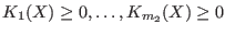 .
There are two phases in the simplex method: phase I verifies if a
feasible solution exists and phase II is used to determine the
extremum of the linear function.
.
There are two phases in the simplex method: phase I verifies if a
feasible solution exists and phase II is used to determine the
extremum of the linear function.
In our case we may use only phase I or phase I and II
by considering the  optimum problems which are to
determine the minimum and maximum of the unknowns under the
optimum problems which are to
determine the minimum and maximum of the unknowns under the
 constraints
 and update the interval for an
unknown if the simplex applied to minimize or maximize enable to
improve the range. It may be seen that this is a
recursive procedure: an improvement on one variable change the
constraint equations and may thus change the result of the simplex
method applied for determining the extremum of a variable which has
already been considered.
and update the interval for an
unknown if the simplex applied to minimize or maximize enable to
improve the range. It may be seen that this is a
recursive procedure: an improvement on one variable change the
constraint equations and may thus change the result of the simplex
method applied for determining the extremum of a variable which has
already been considered.
This procedure, proposed in [25],
enable to correct one of the drawback of the general
solving procedures: each equation is considered independently and for
given intervals for the unknowns two equations may have an interval
evaluation that contain 0 although these equations cannot be canceled
at the same time.
The previous method enable to take into account at least partly the
dependence of the equations. Clearly it will more efficient if the
functions has a large number of linear terms and a "small" non-linear
part.
In all of the following procedures the various storage mode and
bisection mode of the general solving procedures may be used and
inequalities are handled.
The procedure is implemented as:
int Solve_Simplex(int m,int n,int NbNl,
        INTEGER_VECTOR TypeEq,
        INTERVAL_VECTOR (* IntervalFunction)(int,int,INTERVAL_VECTOR &),
        void (* NonLinear)(INTERVAL_VECTOR &x,INTERVAL_VECTOR &X),
        void (* CoeffLinear)(MATRIX &U),
        double MaxDiam,
        int FullSimplex,
        INTERVAL_VECTOR & TheDomain,
        int Order,int Iteration,int Stop,
        double epsilon,double epsilonf,double Dist,
        INTERVAL_MATRIX & Solution,int Nb,
        int (* Simp_Proc)(INTERVAL_VECTOR &))
the arguments being:
- m: number of unknowns
- n: number of equations, see the note 2.3.4.1
- NbNl: number of equations that have no linear term at
all or are inequalities.
If you omit this parameter its value will be assumed to be 0 and
you have to omit the TypeEq parameter.
- TypeEq: an array of integers that indicate the type for
the equations. TypeEq(i) is -1,0,1 if equation i is an
inequality
 , an equation or an inequality
  .
.
- IntervalFunction: a function which return the interval
vector evaluation of the equations, see the note 2.3.4.3 on how
to write this procedure. The equations must be ordered: first
the equations with linear terms then the equations
without any linear terms and finally the inequalities
- NonLinear: a procedure to compute the non linear part of
the equations, see note 2.14.2.1
- CoeffLinear: a procedure that return a matrix which
contain the constant coefficients of the linear term in the equation,
see note 2.14.2.2
- MaxDiam: the simplex method will not be used on boxes
whose maximal width is lower than this value. Should be set
to 0 or a small value
- FullSimplex: this flag is used to indicate how much we
will
use the simplex method (which may be costly). If set to -1 only the
phase I of the simplex will be used. If set to with , then
the full simplex method will be used recursively on the
 variables having the largest interval width.
- TheDomain: box in which we are looking for
solution of the equations
- Order: the type of order which is used to store the
intervals created during the bisection process. This order may be
either MAX_FUNCTION_ORDER or MAX_MIDDLE_FUNCTION_ORDER. See the note on the order 2.3.4.4.
- M: the maximum number of boxes which may be
stored. See the note 2.3.4.5
- Stop: the possible values are 0,1,2
- 0: the algorithm will look for every solution in TheDomain
- 1: the algorithm will stop as soon as 1 solution has
been found
- 2: the algorithm will stop as soon as Nb solutions
have been found
- epsilon: the maximal width of the solution intervals, see the
note 2.3.4.6
- epsilonf: the maximal width of the equation intervals for
a solution, see the
note 2.3.4.6
- Dist: minimal distance between the middle point of two
interval solutions, see the note 2.3.4.7
- Solution: an interval matrix of size (Nb,m)
which will contained the solution intervals. This list is sorted using
the order specified by Order
- Nb: the maximal number of solution which will be returned
by the algorithm
- Simp_Proc: a user-supplied procedure that take as input
the current box and proceed to some further reduction of
the width of the box or even determine that there is no
solution for this box, in which case it should return
-1 (see note 2.3.3).
Remember that you may use the 3B method to improve the efficiency of
this algorithm (see section 2.3.2).
Note that the Simp_Proc argument may be omitted.
The NonLinear procedure
The purpose of the procedure is to compute an interval evaluation of
the non linear term of the equations (the terms in the
mathematical background). This procedure take as argument a box
and the returned evaluation of the non-linear terms.
Consider for example the equations:
The non-linear terms of these equations are
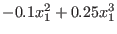 and
and
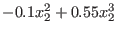 and the NonLinear procedure is
written as:
and the NonLinear procedure is
written as:
void NonLinear(INTERVAL_VECTOR &x,INTERVAL_VECTOR &X)
{
    X(1) = (-0.1+0.25*x(1))*Sqr(x(1));
    X(2) = (-0.1+0.55*x(2))*Sqr(x(2));
}
The CoeffLinear procedure
This procedure returns a matrix  of dimension n m+1 with
  equal to the coefficient of
  in the equation
while
in the equation
while
 is the constant term of the equation. In
the previous example this procedure will be:
is the constant term of the equation. In
the previous example this procedure will be:
void CoeffLinear(MATRIX &U)
{
U(1,1)=1; U(1,2)=0.5; U(1,3)=0.3;
U(2,1)=2; U(1,2)=-0.5; U(1,3)=0.2;
}
In some case it may be interesting to consider an expansion of the
function around a given point. For example consider the term
with in the range [1,2]: in the simplex method the range
[1,4], for this term
will be added to the non linear part of the equation. But if we
substitute the unknown by a new unknown such that  (hence the range for will be [0,1])
we will get
(hence the range for will be [0,1])
we will get
 we will get an additional linear term
(
we will get an additional linear term
( ) while the non linear part will be
  with the range
[0,1]. For each variable
with the range
[0,1]. For each variable  in the range
![$[\underline{y_i},\overline{y_i}]$](img380.png) we may define a new variable
we may define a new variable
 such that
 where has the
range
where has the
range
![$[0,\overline{y_i}-\underline{y_i}]$](img383.png) . We may then write the non
linear and linear procedures for the unknowns but it necessary
to notify the simplex procedure that such an expansion is used. This
is done by setting the flag
ALIAS_Simplex_Expanded to 1 (this possibility is available
only for the simplex method using the gradient).
. We may then write the non
linear and linear procedures for the unknowns but it necessary
to notify the simplex procedure that such an expansion is used. This
is done by setting the flag
ALIAS_Simplex_Expanded to 1 (this possibility is available
only for the simplex method using the gradient).
You may also prohibit the use of the simplex method in the procedure
(for example to use it only in your own simplification procedure) by
setting the flag ALIAS_DONT_USE_SIMPLEX to 1.
The main program for the previous system of 2 equations
(omitting the procedure F that computes the interval evaluation
of the equations) will be
written as
int main()
{
int num,i;
INTERVAL_MATRIX Solution(100,2);
INTERVAL_VECTOR x(2);
INTEGER_VECTOR Type(2);

Clear(Type);
for(i=1;i<=2;i++)x(i)=INTERVAL(-10,10);
Single_Bisection=1;
num=Solve_Simplex(2,2,0,Type,F,NonLinear,CoeffLinear,0.001,0,x,
		  0,40000,0,0.,0.0001,0.0001,Solution,100);

for(i=1;i<=num;i++)
  {
    x(1)=Solution(i,1);x(2)=Solution(i,2);
    cout<<"Solution "<<i<<":"<<x<<endl;
  }
}
This procedure may be used if the gradient of the equations are
available. A full version is implemented as:
int Solve_Simplex_Gradient(int m,int n,int NbNl,
        INTEGER_VECTOR TypeEq,
        INTERVAL_VECTOR (* IntervalFunction)(int,int,INTERVAL_VECTOR &),
        INTERVAL_MATRIX (* Gradient)(int, int,INTERVAL_VECTOR &),
        void (* NonLinear)(INTERVAL_VECTOR &x,INTERVAL_VECTOR &X),
        void (* GradientNonLinear)(INTERVAL_VECTOR &x,INTERVAL_MATRIX &X),
        void (* CoeffLinear)(MATRIX &U),
        double MaxDiam,
        int FullSimplex,
        INTERVAL_VECTOR & TheDomain,
        int Order,int Iteration,int Stop,
        double epsilon,double epsilonf,double Dist,
        INTERVAL_MATRIX & Solution,
        int Nb,int UseGradNL,
        INTEGER_MATRIX &GI,
        int (* Simp_Proc)(INTERVAL_VECTOR &))
the arguments being:
- m: number of unknowns
- n: number of equations, see the note 2.3.4.1
- NbNl: number of equations that have no linear term at
all or are inequalities.
- TypeEq: an array of integers that indicate the type for
the equations. TypeEq(i) is -1,0,1 if equation i is an
inequality , an equation or an inequality .
- IntervalFunction: a function which return the interval
vector evaluation of the equations, see the note 2.3.4.3 on how
to write this procedure. The equations must be ordered: first
the equations with linear terms then the equations
without any linear terms and finally the inequalities
- Gradient: a procedure which return the Jacobian matrix of
the system for given values of the unknowns (see note 2.4.2.2)
- NonLinear: a procedure to compute the non linear part of
the equations, see note 2.14.2.1
- GradientNonLinear: a procedure that returns the gradient
of the non linear part of the equations, see note 2.14.3.1
- CoeffLinear: a procedure that return a matrix which
contain the constant coefficients of the linear term in the equation,
see note 2.14.2.2
- MaxDiam: the simplex method will not be used on boxes
whose maximal width is lower than this value. Should be set
to 0 or a small value
- FullSimplex: this flag is used to indicate how much we
will
use the simplex method (which may be costly). If set to -1 only the
phase I of the simplex will be used. If set to with , then
the full simplex method will be used recursively on the
variables having the largest interval width.
- TheDomain: box in which we are looking for
solution of the equations
- Order: the type of order which is used to store the
intervals created during the bisection process. This order may be
either MAX_FUNCTION_ORDER or MAX_MIDDLE_FUNCTION_ORDER. See the note on the order 2.3.4.4.
- M: the maximum number of boxes which may be
stored. See the note 2.3.4.5
- Stop: the possible values are 0,1,2
- 0: the algorithm will look for every solution in TheDomain
- 1: the algorithm will stop as soon as 1 solution has
been found
- 2: the algorithm will stop as soon as Nb solutions
have been found
- epsilon: the maximal width of the solution intervals, see the
note 2.3.4.6
- epsilonf: the maximal width of the equation intervals for
a solution, see the
note 2.3.4.6
- Dist: minimal distance between the middle point of two
interval solutions, see the note 2.3.4.7
- Solution: an interval matrix of size (Nb,m)
which will contained the solution intervals. This list is sorted using
the order specified by Order
- Nb: the maximal number of solution which will be returned
by the algorithm
- UseGradNL: if set to 1 the algorithm will use the gradient
of the non linear part of the equations to improve their interval
evaluation. Otherwise must be set to 0.
- GI: an integer matrix which give a-priori information on
the sign of the derivative of the function. GI(i,j) indicates
the sign of the derivative of function i with respect to
variable j using the following code:
- -1: the derivative is always negative
- 0: the function is not dependent of variable j
- 1: the derivative is always positive
- 2: the sign of the derivative is not known
- Simp_Proc: a user-supplied procedure that take as input
the current box and proceed to some further reduction of
the width of the box or even determine that there is no
solution for this box, in which case it should return
-1 (see note 2.3.3).
Remember that you may use the 3B method to improve the efficiency of
this algorithm (see section 2.3.2).
The following variables play also a role in the computation:
- ALIAS_Store_Gradient: if not 0 the gradient matrix of
each box will be stored together with the boxes.
Must be set to 0 for large problem
(default value: 1)
- ALIAS_Diam_Max_Gradient: if the maximal width of the
ranges in
a box is lower than this value, then the
gradient will be used to perform the interval evaluation of the
functions (default value: 1.e10)
- ALIAS_Diam_Max_Kraw: if the maximal width of the
ranges in a box is lower than this value, then the
Krawczyk operator will be used to determine if there is a unique
solution in the box (default value: 1.e10)
- ALIAS_Diam_Max_Newton: if the maximal width of the
ranges in a box is lower than this value, then the
interval Newton method will be used either to try to reduce
the width of the box or to to ensure that there is no solution of the
system in the box (default value: 1.e10)
- Min_Diam_Simplex: if the maximal width of the input box
is lower than this value, then the simplex
method will be used
- Max_Diam_Simplex: if the maximal width of the input box
is lower than this value, then the simplex
method will not be used
- Min_Improve_Simplex: when applying the simplex method if
the change on one variable is larger than this value, then the
simplex method will be repeated
- ALIAS_Simplex_Expanded: if set to 1 the expression has
been expanded with respect to the lower bound of each variable
There are several versions of this procedure in which several
arguments of the general procedure may be omitted. The following table
indicates which arguments may be omitted and the corresponding
assumptions (EO=equations only).
|
omitted |
|
|
|
|
|
|
|
NbNl |
|
0 |
|
0 |
|
0 |
|
TypeEq |
EO |
EO |
EO |
EO |
EO |
EO |
|
GradientNonLinear |
|
|
not known |
|
|
not known |
|
UseGradNL |
|
|
0 |
0 |
0 |
0 |
The GradientNonLinear procedure
The purpose of this procedure is to compute the jacobian of the non
linear part of the equations in order to improve their interval
evaluation. The syntax of this procedure is:
void GradientNonLinear(INTERVAL_VECTOR &x,INTERVAL_MATRIX &J)
where x is an interval vector which contains the range for the
unknowns and J is the corresponding jacobian interval matrix.
Solving systems with determinants
In some cases systems may involve determinants: for example in
algebraic geometry the resultant of two algebraic equations is defined
as the determinant of the Sylvester matrix. To get an analytical form
of the equations it is therefore necessary to compute the
determinant: but in some cases this may be quite difficult as the
expression may be quite large, even for sparse matrix. A mechanism in
ALIAS enable to get the interval evaluation of an equation
which include determinant without having to provide the analytical
form of the determinant but only the interval evaluation of the
components of the matrix. This mechanism is based on procedures that
compute the interval evaluation of the determinant of an
interval-valued matrix (see section 7.1).
Using these procedures it is possible to design the equation
evaluation procedure that are used in the general solving procedure of
ALIAS as described in 2.3.4.3. Assume for example that
you have to evaluate the
expression
where A, B are two matrices of dimension 6.
Assume that V is an interval vector which contain the interval
values for and that you have to return the interval evaluation
of this equation in a interval vector W. Then you may write the
following procedure:
INTERVAL_MATRIX A(6,6),B(6,6);
A=Compute_A(V) //compute A for the interval value of x,y
B=Compute_B(V) //compute B for the interval value of x,y
W(1)=(V(1)+Medium_Determinant(A))*V(2)+2*(V(2)+Medium_Determinant(B));
You must be however careful when using this procedure in a denominator
as the presence of 0 in the interval evaluation of the determinant is
not checked, which will
lead to an error when computing the interval evaluation of an
equation (see section 2.1.1.3).
Note that the MakeF procedure of the ALIAS-Maple package
is able to produce efficient code for an equation file even if
unexpanded determinants are present in the equation.
There are also procedures to compute the derivatives of a determinant
Note that the MakeJ procedure of the ALIAS-Maple package
is able to produce a procedure compatible with the requirements of the
gradient procedure required by the library (see
section 2.4.2.2) even if determinants are
present in the equation.
There are also procedures to compute the
second order derivatives of a determinant
Note that the MakeH procedure of the ALIAS-Maple package
is able to produce a procedure compatible with the requirements of the
hessian procedure required by the library (see section 2.5.2.1)
even if determinants are
present in the equation.
Solving systems of distance equations
We consider here a special occurrence of quadratic equations that
describe distances between points in an dimensional space.
Each equation in such system may be written as:
where are unknowns (representing coordinates
of points) and may be unknowns of constants.
A special occurrence of unknowns are the virtual points: the
coordinates
of these points are linear combination of the coordinates of the
points that are defined as the unknowns of the system. To illustrate
the concept of virtual points consider 5 fixed points on a rigid body in the
3-dimensional space. The coordinates of any of this point may be
expressed as a linear combination of the coordinates of the 4 other
points (as soon as these point are not coplanar). The concept of
virtual points has been introduced to allow a decrease in the number
of unknowns but also because without them distance equations will be
redundant and consequently the jacobian of the system of equations
will be singular at a solution thereby prohibiting us of using the
tests (such as Moore or Kantorovitch) that allows to determine that
there is one unique solution in a
given box.
Equations involving
virtual points may be written as:
where the are unknowns and the  unknowns or constants.
Clearly system involving distance equations are of great practical
interest and ALIAS offers a specific algorithm to deal with such
type of systems.
unknowns or constants.
Clearly system involving distance equations are of great practical
interest and ALIAS offers a specific algorithm to deal with such
type of systems.
The method proposed in ALIAS to solve this type of systems is
based on the general procedure using the gradient and hessian. A first
difference is that it is not necessary to provide the gradient and
hessian function as they are easily derived from the system of
equations. Note also that due to the particular structure of the
distance equations the interval evaluation leads to exact bounds.
Furthermore
the algorithm we propose uses a special version of Kantorovitch
theorem (i.e. a version that produces a larger ball with a unique
solution in it compared to the general version of the theorem),
an interval Newton method, a specific version of the simplex method
described in section 2.14 and a specific version of
the inflation method described in section 3.1.6 (i.e. a
method that allows to compute directly the radius of a ball around a
solution that will contain only this solution). In addition two
simplification rules are used:
- as each function is a sum of square term each of them involving
different unknowns we verify if the interval evaluation of the term
has a positive part (in the opposite case the current box
is discarded) and we may update the unknowns so that the negative part
of the term is reduced (this is basically an application of the
concept of 2B-consistency). Hence the procedures described in
section 2.17 should not be used for distance equations.
- based on the triangle equation: each subset of equations
describing the distances between a set of 3 points is detected and the
algorithm verify if the triangle equation is satisfied and, in some
cases may update the boxes.
The algorithm returns as solution either boxes that satisfy
Kantorovitch theorem and therefore are reduced to a point or boxes
such that the function evaluations include 0 and have a width
lower than a given threshold.
A system of distance functions
has a specific description. First
consider distance function that involve only points of constant. Such
function may be written as:
where the maximal number of square term is
and is described by a row of 2 matrices APOW, ACONS
and a vector LI. APOW is an integer matrix with columns and rows
that contain the unknown number
of each term in the function and in which a 0 means that the unknown
is a constant. The value of theses constants are given in the matrix
of real ACONS of size  .
Finally the value of the constant
.
Finally the value of the constant  is
indicated in the vector LI of size . For example consider a system
involving the 4 unknowns
is
indicated in the vector LI of size . For example consider a system
involving the 4 unknowns
 numbered from 1 to 4:
In that case APOW, ACONS, LI will be:
The two first elements of the first row of APOW (1, 0) describes the
first square term of the first equation and state that it is
 , the value of
  being given in the ACONS(1,2). Note that each square term must be written as
(unknown-unknown or constant
being given in the ACONS(1,2). Note that each square term must be written as
(unknown-unknown or constant and not as (constant -unknown.
Consider now function involving virtual points. Each square term may
thus be written as:
where may be either a constant, an unknown or the coordinate of
a virtual point. Let be the number of term of the form
 existing in the system.
Such equation is described by a matrix AVARV with rows and a number of columns equal to the number of
unknowns. Each term
is numbered from 1 to k and
the row of AVARV will contain in position the value of
existing in the system.
Such equation is described by a matrix AVARV with rows and a number of columns equal to the number of
unknowns. Each term
is numbered from 1 to k and
the row of AVARV will contain in position the value of
 . The existence of the coordinate of
a virtual point in a
distance function will be indicated in APOW by a negative number
whose opposite is the number of the virtual coordinates.
Hence if we add to the previous system the third equation:
. The existence of the coordinate of
a virtual point in a
distance function will be indicated in APOW by a negative number
whose opposite is the number of the virtual coordinates.
Hence if we add to the previous system the third equation:
the third row of APOW will be (-1 0 -2 0), the third row of ACONS will be (0 3 0 1) and the third row of LI will be
-10. AVARV will have 2 row and 4 columns and is given as:
Among the equations there will be  equations involving virtual
points. The system must be written in such way that first are defined
the
equations involving virtual
points. The system must be written in such way that first are defined
the  equations not involving virtual points and then the
equations. Note also that in the current implementation
inequalities are handled although with less efficiency than
equations.
The algorithm is implemented as:
equations not involving virtual points and then the
equations. Note also that in the current implementation
inequalities are handled although with less efficiency than
equations.
The algorithm is implemented as:
int Solve_Distance(int DimVar,int DimEq,
                   INTEGER_VECTOR &Type_Eq,
                   INTEGER_MATRIX &APOW,MATRIX &ACONS,VECTOR &LI,
                   int p,int k,MATRIX &AVARV,
                   INTERVAL_VECTOR & TheDomain,
                   int M,
                   double epsilonf,
                   int Stop,
                   INTERVAL_MATRIX & Solution,int Nb,
                   int (* Simp_Proc)(INTERVAL_VECTOR &))
The arguments are:
- DimVar: number of unknowns
- DimEq: number of equations and inequalities in the system
- Type_Eq: an integer array of dimension DimEq where
the j-th element indicates if the j-th function is an equation (value
=0), an inequality (value = -1) or an inequality
(value = 1)
- p: number of functions involving virtual points
- k: number of virtual points
- TheDomain: box in which we are looking for
solution of the system
- M: the maximum number of boxes which may be
stored. In the algorithm we use the reverse storage mode except if the
global integer ALIAS_Parallel_Slave is set
to 1
(its default value is 0)
- epsilonf: either the maximal width of the function intervals for
a solution if it is not determined by using
Newton scheme or the accuracy used in the Newton scheme
- Stop: the possible values are 0,1,2
- 0: the algorithm will look for every solution in TheDomain
- 1: the algorithm will stop as soon as 1 solution has
been found
- 2: the algorithm will stop as soon as Nb solutions
have been found
- Solution: an interval matrix of size (Nb,m)
which will contained the solution intervals. This list is sorted using
the order specified by Order
- Nb: the maximal number of solution which will be returned
by the algorithm
- Simp_Proc: a user-supplied procedure that take as input
the current box and proceed to some further reduction of
the width of the box or even determine that there is no
solution for this box, in which case it should return
-1 (see note 2.3.3).
Remember also that you may use the 3B method to improve the efficiency of
this algorithm (see section 2.3.2).
The argument Simp_Proc in this procedure may be omitted.
The following variables play also a role in the computation:
- ALIAS_Diam_Max_Kraw: if the maximal width of the
ranges in a box is lower than this value, then the
Krawczyk operator will be used to determine if there is a unique
solution in the box (default value: 1.e10)
- ALIAS_Diam_Max_Newton: if the maximal width of the
ranges in a box is lower than this value, then the
interval Newton method will be used either to try to reduce
the width of the box or to to ensure that there is no solution of the
system in the box (default value: 1.e10)
- ALIAS_Permute_List: if the value of this flag is the
algorithm will permute the current list with the largest box in the
list of boxes to process (as the algorithm uses systematically the
Newton scheme with as initial guess the center of the current box
permutation may allow to find quickly new solutions)
This procedure will return:
 : number of solutions
- -1: storage space exceeded
- -2: DimVar or DimVar is a negative number
- -4: an element in Type_Eq is not 0, -1 or 1
- : in the mixed bisection mode the number of variables
that will be bisected is larger than the number of unknowns
- : one of the value of ALIAS_Delta3B or
ALIAS_Max3B is negative or 0
- : one of the value of ALIAS_SubEq3B is not 0 or 1
- : although ALIAS_SubEq3B has as size the number of
equations none of its components is 1
- : ALIAS_ND is different from 0 (i.e. we are
dealing with a non-0 dimensional problem, see the corresponding
chapter) and the name of the result file has not been specified
Note that in this procedure we use the single bisection mode (we
actually select the largest variable as the one that will be bisected)
and the reverse storage mode.
For the distance equations we use a specific procedure for the
inflation method (see section 3.1.6). Indeed in that case it
is possible to calculate directly the diameter of the largest ball
centered at an approximation of a solution that contains one and only
one solution. The procedure is:
int ALIAS_Epsilon_Inflation(int Dimension,int Dimension_Eq,
      INTEGER_MATRIX &APOW,MATRIX &ACONS,
      VECTOR &LI,
      int NB_EQV,int NB_VARV,MATRIX &AVARV,
      VECTOR &Amid,
      INTERVAL_VECTOR &P,
      INTERVAL_VECTOR &PP1,
      int type,double epsilon,
      int (* Simp_Proc)(INTERVAL_VECTOR &))
We have also a specific implementation of the Newton scheme:
int Newton_Fast(int Dimension,int Dimension_Eq,
                   INTEGER_MATRIX &APOW,MATRIX &ACONS,VECTOR &LI,
                   int NB_EQV,int NB_VARV,MATRIX &AVARV,
                   VECTOR &Input,double Accuracy,int Max_Iter,VECTOR &Residu)
For the best efficiency the unknowns has to be well chosen, especially
so that the jacobian of the system has full rank at a solution. The
use of virtual point should be systematic to avoid having a system
that is singular at a solution.
Initial domain and simplification procedures
A specific procedure Bound_Distance
for
finding an initial estimate of the search
domain has been implemented in the ALIAS-Maple
package (
see the ALIAS-Maple manual): this procedure may provide an initial guess
for the solution ranges or improve a given guess.
Note also that the choice of the right coordinate system (for example
its origin) and which points should be defined as virtual points may
have a large influence on the computation time (see an example
in [10]).
Filtering a system of equation
As mentioned previously the 2B heuristic to improve the solving is to
rewrite each equation as the equality of two different terms, to
determine if the interval evaluation of both terms are consistent and
if not to adjust the interval for one term and by using the inverse
function for this term to improve the width for one or more unknowns.
For example imagine that one of the equation is
 . The procedure will introduce a new variable
  such
that
such
that  and compute its interval evaluation. If has a
negative upper bound the equation has no solution for the current
range for . If the upper bound of
is positive then the inverse function of indicates that should
lie in
and compute its interval evaluation. If has a
negative upper bound the equation has no solution for the current
range for . If the upper bound of
is positive then the inverse function of indicates that should
lie in
![$[-\sqrt{U},\sqrt{U}]$](img408.png) : we may then update the interval for
if this is not
the case. If the lower bound of
is positive then the inverse function of indicates that should
lie outside
: we may then update the interval for
if this is not
the case. If the lower bound of
is positive then the inverse function of indicates that should
lie outside
![$[-\sqrt{V},\sqrt{V}]$](img409.png) . If the range for is included
in this interval, then there is no solution to the equation for this
range for .
. If the range for is included
in this interval, then there is no solution to the equation for this
range for .
Note:
- this 2B consistency is implemented in ALIAS-Maple by the
procedure HullConsistencyStrong
- the HullConsistency procedure of ALIAS-Maple may seem to
be redundant with HullConsistencyStrong. This is not the case as
HullConsistency implements a simplification of the left hand
term of the equation that is not performed by HullConsistencyStrong. For example for the equation
 HullConsistencyStrong will rewrite the equation as
 while HullConsistency will use
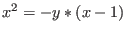 which will lead to a better interval evaluation of
the left hand term
which will lead to a better interval evaluation of
the left hand term
These procedures must not be used with distance equations as
the 2B filtering is already implemented in the solver.


 Next: Analyzing systems of equations
Up: ALIAS-C++
Previous: Introduction
Next: Analyzing systems of equations
Up: ALIAS-C++
Previous: Introduction
![\begin{eqnarray*}
&&X+Y= [\underline{x}+\underline{y},\overline{x}+\overline{y}]\\
&&X-Y= [\underline{x}-\overline{y},\overline{x}-\underline{y}]
\end{eqnarray*}](img7.png)
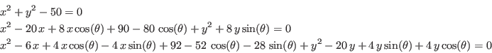
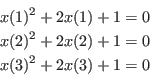
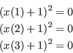
![\begin{eqnarray*}
&&x=[4.99297,4.99902] y=[5.00527,5.01016]
\theta=[-0.00...
...7031] y=[6.21133,6.21621]
\theta=[-0.809942,-0.803806]
\end{eqnarray*}](img172.png)
![\begin{eqnarray*}
&&x=[3.36426,3.37031] y=[6.21621,6.22109]
\theta=[-...
...508,5.01113] y=[4.99063,4.99551]
\theta=[0,0.00613592]
\end{eqnarray*}](img173.png)
![\begin{eqnarray*}
&& {\rm Solution 1}
[4.9990234375,5.005078125]
[4.990625...
...
[6.211328125,6.2162109375]
[-0.809941856,-0.803805932852]
\end{eqnarray*}](img174.png)
![\begin{eqnarray*}
&& \theta=[-0.806784012741056,-0.806781016684830]\\
&& \theta=[-4.793689962142628e-05,0]
\end{eqnarray*}](img182.png)
![\begin{eqnarray*}
&&\psi=[4.661660388259656,4.661660388340929]\\
&&\theta=[1.70...
...00898180284073]\\
&&\phi=[0.869388881899751,0.869388881940387]
\end{eqnarray*}](img189.png)
![\begin{eqnarray*}
&&\psi=[4.661658091884636,4.661658424779772]\\
&&\theta=[1.70...
...00898570395561]\\
&&\phi=[0.869388105618527,0.869388272066095]
\end{eqnarray*}](img190.png)
![\begin{eqnarray*}
&&x=[3.36607,3.37306] y=[6.21468,6.21856] \theta
=[-0.808...
...99845,5.00165] y=[4.99845,5.00146] \theta =[-0.000536641,0]
\end{eqnarray*}](img262.png)
![\begin{eqnarray*}
R&=&
\frac{F(x_3)}{F(x_2)} S=\frac{F(X_3)}{F(x_1)} T=\f...
...\\
P&=&S[T(R-T)(x_2-x_3)-(1-R)(x_3-x_1)]\\
Q&=&(T-1)(R-1)(S-1)
\end{eqnarray*}](img296.png)