INRIA logo
Christopher Mei
PhD Student
Central Catadioptric Systems
And
SLAM
INRIA logo

I am now a research assistant at the University of Oxford, my new wepage is http://www.robots.ox.ac.uk/~cmei/, you should be redirected in 3 seconds.

DOWNLOAD toolbox

NEW calibration toolbox : no prior knowledge is needed on the camera or mirror parameters and we keep the flexibility of only having to select four points for each calibration grid (we do not have to select each corner individually).

The functions containing the projection model (and Jacobians) are available separately in Matlab and as a C++ class with the associated mex functions. The class is initialised with a file generated during the calibration process. It enables the projection of 3D points but also the lifting of image points to their projective rays.

This new "Omnidirectional Calibration Toolbox" is a complete rewrite of the previous version. It uses some functions from the "Caltech Calibration Toolbox" by Jean-Yves Bouguet.

This page gives an example of a calibration session. These images are available for trying out the toolbox. You can find a calibration grid/pattern here. The projection model used is available here.

The toolbox has been successfully used to calibrate hyperbolic, parabolic, folded mirror, spherical and wide-angle sensors.

IMPORTANT : the calibration parameters are calculated with Matlab coordinates (which start at 1) and not with the C/C++ convention (starting at 0).

I would like to thank the ACFR (Australian Center for Field Robotics) for making available some hyperbolic images, and in particular Alex Brooks.

Projection model and parameters

The projection model used is described here. It is a combination of the unified projection model from Geyer and Barreto and a radial distortion function. This model makes it possible take into account the distortion introduced by telecentric lenses (for parabolic mirrors) and gives a greater flexibility (spherical mirrors can be calibrated).

The calibration will estimate :

  • the extrinsic parameters corresponding to the rotation (quaternion : Qw) and translation (Tw) between the grid and the mirror
  • the parameters describing the mirror shape (xi)
  • the distortion induced by the lens (eg. telecentric) (kc)
  • the intrinsic parameters of the generalised camera : skew (alpha_c), generalised focal lengths (gamma1,gamma2) and principal points (cc)

Calibration session

Startup

Please edit the 'SETTINGS.m' file first.
Start the toolbox in Matlab : 

>>omni_calib_gui


This window will appear :

Startup

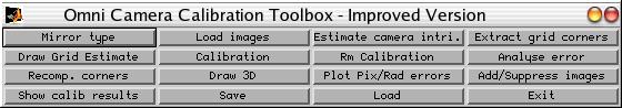
Go to the directory containing the images.
If you would like to know straight away the use of the different buttons, go to this section.

Mirror type


Click on "Mirror type":

1 or [] : parabola (xi=1)
2 : catadioptric (hyperbola,ellipse,sphere)
3 : dioptric (fisheye)
Choice :
Camera type : parabolic.

This step is only to constrain the minimisation in the parabolic case (xi=1) and to avoid trying to extract the mirror border in the dioptric case.

Loading images


"Load images" will ask you for the base name of the images in the current directory and their format :

>>
.                      Omni_Fixed_Values.m    cameraAvecOmni_00.tif  cameraAvecOmni_02.tif  cameraAvecOmni_04.tif  cameraAvecOmni_06.tif 
..                     Omni_Fixed_Values.mat  cameraAvecOmni_01.tif  cameraAvecOmni_03.tif  cameraAvecOmni_05.tif 

Basename camera calibration images (without number nor suffix): cameraAvecOmni_
Image format: ([]='r'='ras', 'b'='bmp', 't'='tif', 'p'='pgm', 'j'='jpg', 'm'='ppm') t
Loading image 1...2...3...4...5...6...7...
done

Mosaic

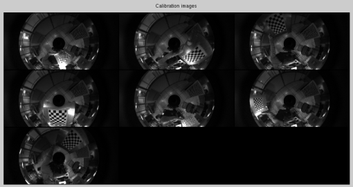
The images are now loaded and we are ready to start estimating the intrinsic values and then calibrating the sensor.

Estimating the intrinsic parameters with the mirror border


By pressing on "Estimate camera intri.", we will calculate an estimate of the intrinsic parameters of the underlying camera (generalised focal length and center).
In the case of a catadioptric sensor, the user is asked to click on the center of the mirror:

Please click on the mirror center and then on the mirror inner border.
Calculating edges... done.
Rejecting inner points... done.
Doing a simplified RANSAC to obtain circle parameters... done.
Was the extraction successful ? ([]=yes, other=no) :

Estimate result

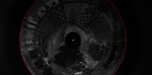
We then estimate the generalised focal length from points on a line image:

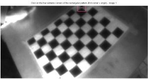
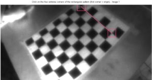
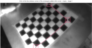
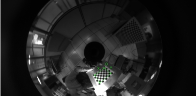
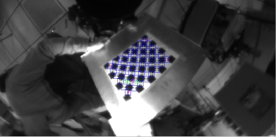
We are now going to estimate the generalised focal (gammac) from line images.
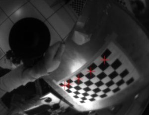
Which image shall we use ? ([] = 1) : 2
Please select at least 4 ALIGNED edge points on a NON-RADIAL line on the grid.
Click with the right button when finished.
done.

Estimate result

Extracting grid corners

We are now ready to extract the grid corners which will be used during the minimisation, press on "Extract grid corners":
Extraction of the grid corners on the images
Number(s) of image(s) to process ([] = all images) =
Window size for corner finder (wintx and winty):
wintx ([] = 8) =  Sub-pixel extraction in the catadioptric case is less tolerant and we should try and keep the window size down.
winty ([] = 8) =
Window size = 17x17

Processing image 1...
Using (wintx,winty)=(8,8) - Window size = 17x17      (Note: To reset the window size, run script clearwin)
Please press enter after zooming...

Extraction

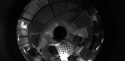
You can now zoom in on the calibration grid and press [ENTER] :

Zoom extraction

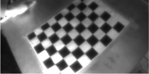
You now need to click on the four corners of the grid in clockwise order :
Point1
Point2
Point3
Point4

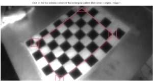
The omni-lines should follow the grid.
You will then be asked for the size of the grid :
Size of each square along the X direction: dX=42mm
Size of each square along the Y direction: dY=42mm   (Note: To reset the size of the squares, clear the variables dX and dY)
Corner extraction...

Result1
Result2

Calibration

Pressing on "Calibration" will start the minimisation :

>>
Aspect ratio optimized (est_aspect_ratio = 1) -> both components of fc are estimated (DEFAULT).
Principal point optimized (center_optim=1) - (DEFAULT). To reject principal point, set center_optim=0
Skew not optimized (est_alpha=0) - (DEFAULT)

Main calibration optimization procedure - Number of images : 7
Gradient descent iterations : WARNING: removing singular matrix warning and managing it internally.
1...2...(r) 3...4...5...6...7...8...9...10...11...12...(r) 13...14...15...16...17...18...19...20...21...22...(r) 23...24...25...26...27...28...29...30...31...32...(r) 33...34...35...36...37...38...39...40...41..
42...(r) 43...44...45...46...47...48...49...50...51...52...(r) 53...54...55...56...57...58...59...Matrix badly conditioned, stopping...
done
Estimation of uncertainties...done


Calibration results after optimization (with uncertainties):

Focal Length:          fc = [17.92581   17.91205 ] ± [ 0.18220   0.21302 ]
Principal point:       cc = [ 980.75605   544.84446 ] ± [ 4.41434   4.64072 ]
Skew:             alpha_c = [ 0.00000 ] ± [ 0.00283  ]   => angle of pixel axes = 90.00000 ± 0.16228 degrees
Distortion:            kc = [ -0.00008   0.00000   0.00000   -0.00000  0.00000 ] ± [ 0.00001   0.00000   0.00003   0.00002  0.00000 ]
Pixel error+-std :          err = [ 0.17324   0.29971 ]+-[ 0.13750   0.24850 ]
Note: The numerical errors are approximately three times the standard deviations (for reference).

Recommendation: The skew coefficient alpha_c is found to be equal to zero (within its uncertainty).
                You may want to reject it from the optimization by setting est_alpha=0 and run Calibration

Recommendation: Some distortion coefficients are found equal to zero (within their uncertainties).
                To reject them from the optimization set est_dist=[1;1;0;0;0] and run Calibration


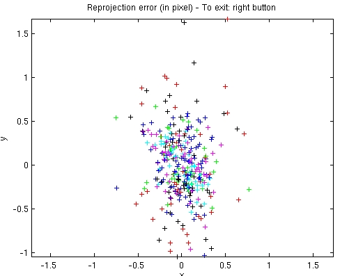
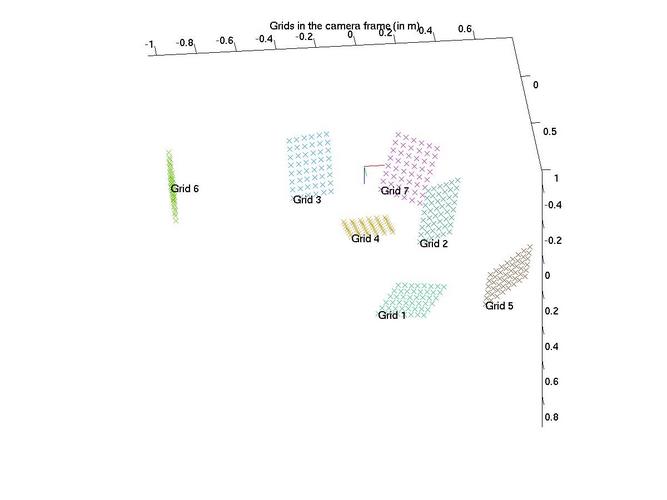
(r) Indicates that the extrinsic parameters are being re-estimated independently.
"Pixel error" is the mean absolute error.


The number of iterations and how often the extrinsic parameters should be computed can be changed in the "SETTINGS.m" file.

Analysing error

Three tools can be used to analyse the error :
  1. "Plot Pix/Rad errors" that gives you the error in the image versus the distance of the points from the image center :

    Error pixels

  2. "Analyse error" this will give you the reprojection error, each color is associated to an image. This will help you identify the points that have been incorrectly extracted.
    You can then reextract corners using "Recomp. corners".

    Analyse error
  3. "Draw 3D" shows the grids in 3D :

    Grids 3D


BEWARE : When calibrating, it is not sufficient to look at the absolute error. The average over all the errors doesn't take into account the spatial distribution of the error . The calibration might then depend on the position of the grids (bias).

Different buttons and settings

The "SETTINGS.m" file contains the path to the toolbox and variables for the minimisation (max. of iterations and step before recomputing the extrinsic parameters).

Buttons :
  • "Mirror type" to input the values of the mirror diameter and parameters
  • "Load images" to load the images used for the calibration
  • "Estimate camera intri." to obtain initial values for the calibration using the mirror border
  • "Extract grid corners" helps extract the grid corners for the calibration
  • "Draw Grid Estimate" projects in yellow the grid points according to the calculated values, in red are the extracted points
  • "Calibration" launches the minimisation using the distance in the image
  • "Rm Calibration" removes the calibration parameters
  • "Analyse error" reprojects the error, this can be used to find images where the points have not been properly extracted
  • "Recomp. corners" recomputes the point extraction after reprojecting the grid points (this can be used when "Analyse Error" shows that some grid points have been incorrectly extracted)
  • "Draw 3D" draws a 3D view of the camera and grids
  • "Plot Pix/Rad errors" plots the error in pixels versus the distance of the points to the image center
  • "Add/Suppress images" makes it possible to add or remove images
  • "Show calib results" show the calibration values and errors
  • "Save" saves the extrinsic and intrinsic parameters, the grid points, ...
  • "Load" loads the values obtained during the calibration
  • "Exit" quits the program

Download

The files that are not part of the "Caltech Calibration Toolbox" by Jean-Yves Bouguet are issued under the GPL license Version 2.

If you have any suggestions, bug corrections please write to : Christopher.Mei@sophia.inria.fr

Improved Omnidirectional Calibration Toolbox (don't forget to change the 'SETTINGS.m' file)
[ZIP] [BZ2]
Projection functions (matlab, C++, mex files) [ZIP][BZ2]
Images to test the calibration toolbox [ZIP][BZ2]
Projection model [PDF]
Calibration grid/pattern [PDF]

Old toolbox

Old toolbox, no longer maintained.


Version 0.93
Matlab Omnidirectional Calibration Toolbox   (don't forget to change the 'SETTINGS.m' file)
[ZIP] [BZ2]
Images to test the calibration toolbox [ZIP][BZ2]

Version 1.1
C program to undistort the images
[ZIP] [BZ2]

Version 1.0
C example program to read the undistorted calibration model
[ZIP] [BZ2]

FAQ

Q : When I call the "Extract grid corners", I get an error "identifier" expected, "(" found." !

Answer : Since version 0.92 (compatible with matlab 6), this shouldn't happen anymore!


Q : I cannot find the 'imshow' function !

Answer : The "imshow" function is part of Matlab's Image Processing Toolbox.