INRIA home page
Subsections
Continuation for one dimensional system
Although mostly devoted to zero-dimensional systems ALIAS still
offers some possibilities to deal with  -dimensional systems. The
purpose of the algorithms here is to consider a system with
parameter and to follow the branches of the solutions of the system
when these parameters are varying between some bounds.
-dimensional systems. The
purpose of the algorithms here is to consider a system with
parameter and to follow the branches of the solutions of the system
when these parameters are varying between some bounds.
Continuation 1D
Let consider a system of equations in  unknowns
 and assume that
  may vary in the range
![$[\underline{x_1},\overline{x_1}]$](img768.png) and that it is considered as the
parameter of this
system. Using the solving algorithms of
ALIAS (or any other
method) we are able to determine the real roots of this system, if any, for a
given value of the parameter, for example for
and that it is considered as the
parameter of this
system. Using the solving algorithms of
ALIAS (or any other
method) we are able to determine the real roots of this system, if any, for a
given value of the parameter, for example for
 . Let
assume that we have found
. Let
assume that we have found  real roots
 . Assume now
that we change the value of to
. Assume now
that we change the value of to
 . Using
Kantorovitch theorem (see section 3.1.2)
we are able to determine if Newton method with as
initial estimate
. Using
Kantorovitch theorem (see section 3.1.2)
we are able to determine if Newton method with as
initial estimate  will converge toward a solution of the new
system and the radius
of convergence
will converge toward a solution of the new
system and the radius
of convergence  such that the solution is unique in the ball
![$B_i =[X_i-\alpha_i, X_i+\alpha_i]$](img774.png) (alternatively we may also use
Moore theorem, see section 2.10).
If this is the case and if the
intersection of the
(alternatively we may also use
Moore theorem, see section 2.10).
If this is the case and if the
intersection of the  is empty, then we are able to compute in a
certified way the new solutions of the new system. Otherwise we
will repeat the procedure with a smaller value for
is empty, then we are able to compute in a
certified way the new solutions of the new system. Otherwise we
will repeat the procedure with a smaller value for  until
the method succeed. A failure case will be when the system become
singular at a point (for example when 2 branches are collapsing). If
this happen we will change the value of
until we find a new set of solutions
which satisfy Kantorovitch theorem and start again the process.
until
the method succeed. A failure case will be when the system become
singular at a point (for example when 2 branches are collapsing). If
this happen we will change the value of
until we find a new set of solutions
which satisfy Kantorovitch theorem and start again the process.
This method enable to follow all the branches for which initial points have
been found when solving the initial system. We may then store these
points in an array, for example at regular step for the value
of the parameter.
By default we use Kantorovitch theorem to follow the branches but by
setting the global variable
ALIAS_Use_Kraw_Continuation
to 1 we will use Moore test.
The procedure that allow to determine the next point on a branch is
implemented as:
int Certified_Newton(int Nb_Var,int Dimension_Eq,int Nb_Branch,int Branch,
                       INTERVAL_VECTOR (* Func)(int,int,INTERVAL_VECTOR &),
                       INTERVAL_MATRIX (* Gradient)(int, int,INTERVAL_VECTOR &),
                       INTERVAL_MATRIX (* Hessian)(int, int, INTERVAL_VECTOR &),
                       double Accuracy_Var,double Accuracy,
                       double *param,double delta_param,double min_delta_param,
                       int sens,MATRIX &Solution)
This procedure determine if it possible to find a new point on the
branch numbered Branch among the Nb_Branch that have been
found. In Solution we have all the solutions that have been
found for the branches when the parameter value was param. The
change in the parameter value will be at most sens delta_param and
on exit of the procedure param will be set to the new
value. sens indicates the direction of change in the parameter
value: +1 for an increase, -1 for a decrease.
delta_param and
on exit of the procedure param will be set to the new
value. sens indicates the direction of change in the parameter
value: +1 for an increase, -1 for a decrease.
This procedure returns:
- -1, -4: even with a change of the parameter value of min_delta_param we cannot either distinguish two solutions or
Kantorovitch has failed to give a positive answer. But this does not
mean in general that a singularity occurs.
- -2: for systems having more equations than unknowns the solution
that has been obtained with Newton for the square system of equations
failed to cancel the remaining equations
- -3: Newton has not converged (should not occur)
- -10: singular point
- 1, 2: procedure has succeeded
This procedure takes as input a set of solutions of the system and
will return points on the branches. The branches will be followed
until a given value for the parameter is reached or if Kantorovitch
theorem is no more satisfied for some value of the parameter.
It is implemented as:
int ALIAS_Start_Continuation(int m,int n,int NUM,
       INTERVAL_MATRIX &Solutions,
       INTERVAL_VECTOR (* IntervalFunction)(int,int,INTERVAL_VECTOR &),
       INTERVAL_MATRIX (* Gradient)(int, int,INTERVAL_VECTOR &),
       INTERVAL_MATRIX (* IntervalHessian)(int,int,INTERVAL_VECTOR &),
       double epsilon,double epsilonf,
       double *z,double delta,double mindelta,
       INTERVAL &Rangez,
       int sens,
       MATRIX &BRANCH,int *NBBRANCH)
the arguments being:
- m: number of unknowns
- n: number of equations
- NUM: the number of solutions of the system for the current
value of the parameter z
- Solutions: the solutions of the system for the current
value of the parameter z
- IntervalFunction: a function which return the interval
vector evaluation of the equations, see
note 2.3.4.3.
- IntervalGradient: a function which return
the interval matrix of the
jacobian of the equations, see note 2.4.2.2
- IntervalHessian: a function which return
the interval matrix of the
Hessian of the equations, see note 2.5.2.1
- epsilon: the maximal width of the box, see the
note 2.3.4.6. If all the variable ranges have a width lower than
this value and the interval evaluation of the equations contains all
0, then the set of ranges is considered to be a solution. But they
will be not considered as a valid solution as they will not satisfy
Kantorovitch theorem. Hence you must put here a very small value
- epsilonf: the maximal width of the equation intervals, see the
note 2.3.4.6. This value will be used by the iterative Newton
scheme to stop the iteration.
- z: the parameter of the system
- delta: if
 is the first value of the parameter such
that the system has solutions, then we will store in BRANCH the
solutions for +delta, +2delta,...
is the first value of the parameter such
that the system has solutions, then we will store in BRANCH the
solutions for +delta, +2delta,...
- mindelta: if the algorithm is unable to find a
Kantorovitch solution for the parameter value z+mindelta while a
solution has been found for z, then the algorithm will assume
that we are close to a singular point. Hence mindelta should
have a small value
- Rangez: the range for the parameter z
- sens: either 1 or -1. If 1 the branch will be computed for
increasing values of z, if -1 for decreasing values of z. This parameter should be chosen according to the largest number of
solutions of the system for the lower and upper value of z
- BRANCH: the procedure will return an array of NBBRANCH lines and m+2 columns, which describe the points of
the branch. In a line the first m+1 elements are the coordinates
of the point and the m+2 elements is the number of the branch to
which belong this point. The points are not ordered with respect to
the branch number. The algorithm will take care of resizing BRANCH as needed, hence there is no need to give dimension for this parameter
- NBBRANCH: the total number of points in the array BRANCH.
The return code is:
- 1: the branches have been successfully determined
- -1, -2: the algorithm has failed to find a Kantorovitch solution
for the current value of the parameter
- -3: failure in Newton method (should not occur)
- -10: for the current value of the parameter the jacobian is
singular
- -20: sens is not 1 or -1
- -30: delta or mindelta is negative
Even for a negative return code the points in BRANCH are valid:
the procedure will return the points that have computed on the
branches but is simply not able
to determine the location of new branches that may have appeared.
Full continuation procedure
This procedure will determine initial points on the branches of the
system for the value
of the parameter within some bounds and then follow the branches. It
is implemented as
int ALIAS_Full_Continuation(int m,int n,
       INTERVAL_VECTOR (* IntervalFunction)(int,int,INTERVAL_VECTOR &),
       INTERVAL_MATRIX (* Gradient)(int, int,INTERVAL_VECTOR &),
       INTERVAL_MATRIX (* IntervalHessian)(int,int,INTERVAL_VECTOR &),
       INTERVAL_VECTOR &Domain,
       int M,
       double epsilon,double epsilonf,
       double *z,double delta,double mindelta,double mindz,
       INTERVAL &Rangez,
       int sens,
       MATRIX &BRANCH,int *NBBRANCH)
The arguments are the same than for the previous procedure except for:
- Domain: the range for the m variable in which we will
look for solutions of the system,
- M is the maximum number of boxes which may be
stored (see the note 2.3.4.5)
- mindz: the accuracy
with which the starting point for the branches will be determined: if
the value of the parameter at which the branches will start is ,
then the system has no solution for
 -mindz. This is done
by using a bisection on the parameter: if at
-mindz. This is done
by using a bisection on the parameter: if at  the system has no
solution and has a positive number of solution at +delta,
then we will solve the system for +delta/2. At each time we
will store the value
the system has no
solution and has a positive number of solution at +delta,
then we will solve the system for +delta/2. At each time we
will store the value  of the parameter for which there is no solution
of the system and the value
of the parameter for which there is no solution
of the system and the value  for which we have solutions and we
will stop the bisection on the parameter as soon as
for which we have solutions and we
will stop the bisection on the parameter as soon as  mindz.
To determine the starting points of the branches this procedure uses the
solving procedure with the Hessian (see section 2.5). As
soon as initial valid solutions are
found the ALIAS_Start_Continuation procedure is called until
either a bound of the
parameter range is reached, or a singularity occur. In the later case the
solving procedure is called with an increased value for the
parameter. This algorithm cannot find isolated points and may miss
branches (see next section).
There is also another version of this program where you indicate just
before Domain the solutions which have already been found. The
syntax is
       INTERVAL_MATRIX (* IntervalHessian)(int,int,INTERVAL_VECTOR &),
       int NUM,
       INTERVAL_MATRIX &Solutions,
       INTERVAL_VECTOR &Domain
The return code for these procedures are:
 : the number of branches found by the algorithm
- -1: no initial point have been found
- -10: Newton algorithm has failed (should not occur)
- -20: sens is not 1 or -1
- -30: delta or mindelta is negative
Finding the initial starting point with the accuracy
mindz may be computer intensive.
Hence the integer global variable
ALIAS_Allow_Backtrack
enable to disable this process if it is set to 0 (its default value is
1): in that case as soon as starting points have been found (hence at
+ delta) we will start following the branches.
In fact these procedures are special occurrences of another ALIAS
procedure which has another argument right after the Hessian
argument. Assume for example that you are considering a system which
has one equation written as:
where  is the parameter of the system and
  the
unknowns. When using the continuation method we have to define
ranges for these unknowns in order to be able to solve the system of
equations. Up to now we have indicated bounds that are constants but
for the equation example it will be interesting to be able to specify
that these bounds may change according to the value for the
parameter using a
simplification procedure.
In our example
clearly
the
unknowns. When using the continuation method we have to define
ranges for these unknowns in order to be able to solve the system of
equations. Up to now we have indicated bounds that are constants but
for the equation example it will be interesting to be able to specify
that these bounds may change according to the value for the
parameter using a
simplification procedure.
In our example
clearly  and
and  cannot exceed
  and
cannot be lower than
and
cannot be lower than  (this is an application of the
concept of
2B-consistency, see section 2.17).
Hence we may specify right after the
Hessian argument the name of a procedure, for example Range,
that is able to update
the bounds on the unknowns according to the value of the parameter (or
any other variable that may play a role). The syntax of the procedure
Range
is:
(this is an application of the
concept of
2B-consistency, see section 2.17).
Hence we may specify right after the
Hessian argument the name of a procedure, for example Range,
that is able to update
the bounds on the unknowns according to the value of the parameter (or
any other variable that may play a role). The syntax of the procedure
Range
is:
INTERVAL_VECTOR Range(double z, INTERVAL_VECTOR &Variable)
where z is parameter value and Variable the current set of ranges
for the unknowns. This procedure must return a set of ranges for the
unknowns (be careful to check that the returned ranges are included in
the initial ranges).
Note also that the ALIAS-Maple package offers a procedure that
uses the method described in section 2.14 for finding
the initial starting points of the branches: this method is efficient
if the equations include linear terms in the unknowns.
Clearly there is a major problem with the method we are proposing: we
may miss some branches. For example imagine that a system has
roots for the initial value of the parameter, but will have more than
solutions for another value of the parameter, meaning that
new branches appear: our algorithm will find only the initial
branches. There are two methods that can be used to find the correct
number of branches. The first one is simply to start following the
branches with as initial value for the parameter the one among the
highest or smallest value having led to the maximum number of
solution.
There is also another mechanism that enable to avoid missing
branches. Assume that the solving procedure has determined for some
initial value  of the parameter
solutions to the system and that at some point
of the parameter
solutions to the system and that at some point  the continuation
method has failed: the solving procedure is called and determine that
the system has now
the continuation
method has failed: the solving procedure is called and determine that
the system has now  solutions. This mean that for some parameter
value between and we have missed
solutions. This mean that for some parameter
value between and we have missed  branches. At such point, called problem point it would be
interesting to backtrack i.e. to start again a continuation process
with as initial point for the branches the solutions obtained for
and a value for Sens which
is the opposite of the initial value. This is what
is done by the procedure which may store up to 10 problem points. As
this process may be computer intensive it is possible to disable it by
setting
the integer global variable
ALIAS_Problem_Continuation to -1 (it's default value is 0,
which mean that the process is enabled).
branches. At such point, called problem point it would be
interesting to backtrack i.e. to start again a continuation process
with as initial point for the branches the solutions obtained for
and a value for Sens which
is the opposite of the initial value. This is what
is done by the procedure which may store up to 10 problem points. As
this process may be computer intensive it is possible to disable it by
setting
the integer global variable
ALIAS_Problem_Continuation to -1 (it's default value is 0,
which mean that the process is enabled).
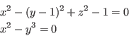
Let consider the system:
The purpose of this example is to write the points of the branches of
this system in files whose name is BRANCH followed by the branch
number.
The main file is written as:
#include "Functions.h"
#include "Vector.h"
#include "IntervalVector.h"
#include "IntervalMatrix.h"
#include "IntegerMatrix.h"
#include "header_Solve_General_Interval.h"
#include "header_Utilities_Interval.h"
double z;
//F,J,H are the equation, jacobian and hessian procedures
#include "F.C"
#include "J.C"
#include "H.C"

int main()
{
MATRIX BRANCH;
INTERVAL RANGE;
int NUM,i,j,NB_BRANCH;
char texte[400];
double delta=0.05;
double min_delta=1.e-6;
double mindz=1.e-4;
ostream out;

int Nb_Var=2;
int Nb_Eq=2;
Domain(1)=INTERVAL(-100,100);
Domain(2)=INTERVAL(-100,100);
RANGE=INTERVAL(0.2);
NUM=ALIAS_Full_Continuation(Nb_Var,Nb_Eq,F,J,H,Domain,1.e-6,1.e-6,&z,
	delta,min_delta,mindz,RANGE,1,BRANCH,&NB_BRANCH);

//order the branch and write the result in the file
for(i =1;i<=NUM;i++)
     {
       sprintf(texte,"BRANCH%d",i);
       out.open(texte,ios::out);
       for(j =1;j<=NB_BRANCH;j++)
          {
           if(BRANCH(j,Nb_Var+2)!=i)continue;
           out<<BRANCH(j,1)<<" "<<BRANCH(j,2)<<" "<<BRANCH(j,3)<<endl;
          }
      out.close();
      }
}


 Next: Integration
Up: ALIAS-C++
Previous: Optimization
Next: Integration
Up: ALIAS-C++
Previous: Optimization