INRIA home page
Subsections
Optimization
ALIAS is also able to deal with optimization problem. Let
consider a scalar function  of
of  variables
 , called the optimum function
and
assume that you are looking for the global minimal or maximal
value of when the
unknowns lie in some ranges.
Furthermore the unknowns may be submitted to
, called the optimum function
and
assume that you are looking for the global minimal or maximal
value of when the
unknowns lie in some ranges.
Furthermore the unknowns may be submitted to  constraints
of type
constraints
of type  ,
,  constraints of type
 and
and  constraints of type
  .
Note that
.
Note that
 may have interval
coefficients.
may have interval
coefficients.
As interval coefficients may appear in the function we have to
define what will be called a minimum or a maximum of . First we
assume that there is no interval coefficients in and denote by
 the minimal or maximal value of over a set of ranges defined
for
the minimal or maximal value of over a set of ranges defined
for  and an accuracy
  with which we want to determine
the extremum. The algorithm will return an interval
with which we want to determine
the extremum. The algorithm will return an interval  as an approximation of such that
for a minimization problem
as an approximation of such that
for a minimization problem
 and
for a maximization problem
and
for a maximization problem
 . The
algorithm will also return a value
. The
algorithm will also return a value  for where the extremum
occurs. If we deal with a constrained optimization problem we will
have:
for where the extremum
occurs. If we deal with a constrained optimization problem we will
have:
where  has a pre-defined value.
Note that if we have constraint equation of type the result
of the optimization problem may be no more guaranteed
as the constraint itself
has a pre-defined value.
Note that if we have constraint equation of type the result
of the optimization problem may be no more guaranteed
as the constraint itself  may not be verified.
If there are interval coefficients in the optimum function there is
not a unique but according to the value of the coefficient a
minimal extremum value  and a maximal extremum value
 . The algorithm will return in the lower bound of an
approximation of and in the upper bound of an
approximation of which verify for a minimization problem:
. The algorithm will return in the lower bound of an
approximation of and in the upper bound of an
approximation of which verify for a minimization problem:
Note that the width of may now be greater than .The
algorithm will return also two solutions  for
corresponding respectively to the values of
for
corresponding respectively to the values of  . If we are
dealing with a constrained optimization problem the solutions will
verify the above constraint equations.
. If we are
dealing with a constrained optimization problem the solutions will
verify the above constraint equations.
If the optimum function has no interval coefficients the algorithm
may return no solution if the interval evaluation of the optimum
function has a width larger than . Evidently the algorithm
will also return no solution if there is no solution that satisfy all
the constraints.
A first method to find all the solutions of an optimum problem
is to consider the system of derivative equations and find its root
(eventually under the given constraints): this may be done with the
solving procedures described in a previous chapter. Hence we have
implemented an alternative method which is able to work even if the
optimum function has, globally or locally, no derivatives.
This method is implemented as a special case of the general
solving procedures. The only difference is that the procedure maintains
a value for the current optimum: during the bisection process we
evaluate the optimum function for each new box and reject those
that are not compatible with the current optimum.
Two types of method enable to solve
an optimization problem:
- a method which need only a procedure for evaluating ,
- a method which need a procedure for evaluating and a
procedure for evaluating its gradient,
Note that with the first method none of the function needs to be
differentiable while for the other one not all the functions in the
set  must be differentiable: only one function in the set
has to be differentiable.
must be differentiable: only one function in the set
has to be differentiable.
For the first method
we update the current optimum by computing the optimum
function value at the middle point of the box. For the
method with the gradient a local optimizer based on the steepest
descent
method is also used if there is
only one equation to be minimized or if there are only inequalities
constraints. The local optimizer works in 2 steps: first a rough
optimization and then a more elaborate procedure if the result of the
first step is better than a fixed threshold defined by the global
variable ALIAS_Threshold_Optimiser
whose default value is 100.
Additionally if an extremum  has been already determined
the local optimizer (which may computer intensive)
is called only if the function value
has been already determined
the local optimizer (which may computer intensive)
is called only if the function value  at the middle
point is such that for a maximum
at the middle
point is such that for a maximum
 and
and
 for a minimum, where ALIAS_LO_A and ALIAS_LO_B are global variables with default
value 0.9 and 1.1.
for a minimum, where ALIAS_LO_A and ALIAS_LO_B are global variables with default
value 0.9 and 1.1.
Implementation
Preliminary notes:
The optimization
method is implemented as:
int Minimize_Maximize(int m,int n,
      INTEGER_VECTOR &Type_Eq,
      INTERVAL_VECTOR (* TheIntervalFunction)(int,int,INTERVAL_VECTOR &),
      INTERVAL_VECTOR & TheDomain,
      int Iteration,int Order,
      double epsilon,double epsilonf,double epsilone,
      int Func_Has_Interval,
      INTERVAL Optimum,
      INTERVAL_MATRIX & Solution,
      int (* Simp_Proc)(INTERVAL_VECTOR &));
the arguments being:
- m: number of unknowns
- n: number of equations, see the note 2.3.4.1
- Type_Eq: type of the equations:
- Type_Eq(i)=-1 if equation i is a constraint
equation of type

- Type_Eq(i)=0 if equation i is a constraint
equation of type

- Type_Eq(i)=1 if equation i is a constraint
equation of type

- Type_Eq(i)=-2 if equation i is the optimum
function to be minimized
- Type_Eq(i)=2 if equation i is the optimum
function to be maximized
- Type_Eq(i)=10 if equation i is the optimum
function for which is sought the minimum and maximum
- IntervalFunction: a function which return the interval
vector evaluation of the equations, see the note 2.3.4.3. This
function must be written in a similar manner than for the general
solving procedures.
Note also that a convenient way to write the IntervalFunction
procedure is to use the possibilities offered by the ALIAS-Maple
(see the ALIAS-Maple manual).
- TheDomain: box in which we are looking for
the extremum of the optimum function
- Iteration: the number of boxes that may be
stored
- Order: a flag describing which order is used to store the
new boxes, see the note 8.3.4
- epsilon: the maximal width of the solution intervals but
not used. Should be set to 0.
- epsilonf: the maximal error for the equality
constraints. If the
problem has constraint of type then a solution will verify
- epsilone: the maximal error on the extremum value.
If the extremum of the function is
 and the procedure
returns the value
and the procedure
returns the value  , then a minimum will verify
 and a maximum
 .
.
- Func_Has_Interval: 1 if the optimum function has
interval coefficients, 0 otherwise
- Optimum: an interval which contain the extremum value of
the optimum function
- Solution: an interval matrix of size at least (2,m)
which will contained the values of for which the extremum are
obtained
- Simp_Proc: an optional parameter which is a
simplification
procedure that may be provided by the user. It takes as input a box
 and may:
- either returns in a box with lower width than the initial
and a return code 0 or 1
- or indicates that there is no solution to the
optimization problem in the current box, in which case the procedure
returns -1
An often efficient simplification procedure is the 2B method (see
section 2.17) that may be automatically generated by the
HullIConsistency procedure of ALIAS-Maple
Thus to minimize a function you have to set its Type_Eq to -2,
to maximize it to set its Type_Eq to 2, while if you are
looking for both a minimum and a maximum Type_Eq should be set
to 10.
Remember that you may use the 3B method to improve the efficiency of
this algorithm (see section 2.3.2) if you have constraint equations.
In some cases it may be interesting to determine if the minimum and
maximum have same sign. This may be done by setting the flag
ALIAS_Stop_Sign_Extremum either to:
- 1: the procedure will return immediately as soon as it is proven
that the extremum will have opposite sign i.e. as soon as two points
lead to opposite value for the function. But if the extremum have
identical sign the minimum and maximum will be computed up to the
accuracy epsilone
- 2: the procedure will return immediately as soon as it is proven
that the extremum will have opposite sign i.e. as soon as two points
lead to opposite value for the function. If the extremum have same
sign the values returned by the procedure are not the minimum and
maximum of the function
With the flag set to 2 the detection that the extremum will have
opposite sign is faster.
The procedure will return an integer  that will be identical to the
code returned by the procedure
that will be identical to the
code returned by the procedure
Solve_General_Interval except for:
 : one of the equation in the system has not a type 0, -1,
-2, 2, 10
or 1 (i.e. it's not an equation or an optimum function,
neither inequality
: one of the equation in the system has not a type 0, -1,
-2, 2, 10
or 1 (i.e. it's not an equation or an optimum function,
neither inequality  or an
inequality
or an
inequality  )
)
 : there is no optimum function i.e. no equation has type
2 or -2 or 10
: there is no optimum function i.e. no equation has type
2 or -2 or 10
 : there is more than one optimum function i.e. more than
one equation has type 2 or -2 or 10
: there is more than one optimum function i.e. more than
one equation has type 2 or -2 or 10
In this version of
ALIAS there is no direct way to deal with inequalities that
are valid for the same function (e.g.
 ), which mean that you will have to declare two inequalities
(which imply that the quantity
), which mean that you will have to declare two inequalities
(which imply that the quantity  will be evaluated twice).
But in the previous procedure there is a way to avoid writing
two inequalities. In the function evaluation procedure you will just
compute
will be evaluated twice).
But in the previous procedure there is a way to avoid writing
two inequalities. In the function evaluation procedure you will just
compute  and declare this function as an inequality of type
. After having computed the interval evaluation
and declare this function as an inequality of type
. After having computed the interval evaluation
- if
this interval is strictly included in
![$[\alpha,\beta]$](img741.png) substitute the interval of by the value -1 (or any negative number)
substitute the interval of by the value -1 (or any negative number)
- if this interval has no intersection with
substitute the interval of by the value 1 (or any positive number)
- if this interval has an intersection with
but
is not strictly included in it, then
substitute the interval of by the interval [-1,1]
The optimization
method is implemented as:
int Minimize_Maximize_Gradient(int m,int n,
      INTEGER_VECTOR &Type_Eq,
      INTERVAL_VECTOR (* TheIntervalFunction)(int,int,INTERVAL_VECTOR &),
      INTERVAL_MATRIX (* Gradient)(int, int,INTERVAL_VECTOR &),
      INTERVAL_VECTOR & TheDomain,
      int Iteration,int Order,
      double epsilon,double epsilonf,double epsilone,
      int Func_Has_Interval,
      INTERVAL Optimum,
      INTERVAL_MATRIX & Solution,
      int (* Simp_Proc)(INTERVAL_VECTOR &));
the arguments being:
- m: number of unknowns
- n: number of equations, see the note 2.3.4.1
- Type_Eq: type of the equations:
- Type_Eq(i)=-1 if equation i is a constraint
equation of type
- Type_Eq(i)=0 if equation i is a constraint
equation of type
- Type_Eq(i)=1 if equation i is a constraint
equation of type
- Type_Eq(i)=-2 if equation i is the optimum
function to be minimized
- Type_Eq(i)=2 if equation i is the optimum
function to be maximized
- Type_Eq(i)=10 if equation i is the optimum
function for which is sought the minimum and maximum
- IntervalFunction: a function which return the interval
vector evaluation of the equations, see the note 2.3.4.3. This
function must be written in a similar manner than for the general
solving procedures.
- Gradient: a function which return the interval evaluation
of the gradient of the equations, see the note 2.4.2.2.
This
function must be written in a similar manner than for the general
solving procedures with the additional constraint that the
function to be minimized of maximized must be the last one.
- TheDomain: box in which we are looking for
the extremum of the optimum function
- Iteration: the number of boxes that may be
stored
- Order: a flag describing which order is used to store the
new boxes, see the note 8.3.4
- epsilon: the maximal width of the solution intervals but
not used. Should be set to 0.
- epsilonf: the maximal error for the equality
constraints. If the
problem has constraint of type then a solution will verify
- epsilone: the maximal error on the extremum value.
If the extremum of the function is and the procedure
returns the value , then a minimum will verify
and a maximum
.
- Func_Has_Interval: 1 if the optimum function has
interval coefficients, 0 otherwise
- Optimum: an interval which contain the extremum value of
the optimum function
- Solution: an interval matrix of size at least (2,m)
which will contained the values of for which the extremum are
obtained
- Simp_Proc: an optional parameter which is a
simplification
procedure that may be provided by the user. It takes as input a box
and may:
- either returns in a box with lower width than the initial
and a return code 0 or 1
- or indicates that there is no solution to the
optimization problem in the current box, in which case the procedure
returns -1
Thus to minimize a function you have to set its Type_Eq to -2
and to maximize it to set its Type_Eq to 2.
Remember that you may use the 3B method to improve the efficiency of
this algorithm (see section 2.3.2).
Note also that a convenient way to write the IntervalFunction
and Gradient
procedures is to use the possibilities offered by ALIAS-Maple
(see the ALIAS-Maple manual).
The procedure will return an integer that will be identical to the
code returned by the procedure
Solve_General_Gradient_Interval except for:
- : one of the equation in the system has not a type 0, -1,
-2, 2, 10
or 1 (i.e. it's not an equation or an optimum function,
neither inequality or an
inequality )
- : there is no optimum function i.e. no equation has type
2 or -2 or 10
- : there is more than one optimum function i.e. more than
one equation has type 2 or -2 or 10
 : the last function is not the one to be minimized or maximized
Note that this implementation is only a special occurrence of the
general solving procedure and thus offer the same possibilities to
improve the storage management (see section 2.4).
Order
During the bisection process new boxes will be created and
stored in the list. But we want to order these new boxes so
that the procedure will consider first the most promising box.
The ordering is based on an evaluation index, the new boxes
being stored using an increasing order of the index (the
box with the lowest index will be stored first).
The flag Order indicate which index is used:
indexMAXCONSTRAINTFUNCTION@MAX_CONSTRAINT_FUNCTION
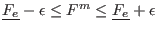
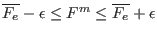
- MAX_FUNCTION_ORDER: let
![$[\underline{F_i},\overline{F_i}]$](img743.png) be the interval evaluation of
the optimum equation
be the interval evaluation of
the optimum equation  . The index is obtained as
 for a minimization problem
and
for a minimization problem
and
 for a maximization problem,
- MAX_CONSTRAINT_FUNCTION: same than MAX_FUNCTION_ORDER if there is only one equation in the system.
Otherwise:
- if there are equality constraints use the
MAX_FUNCTION_ORDER index
- if there are only inequality constraints and if they all
hold for all the new boxes, then the index is the lower bound
of the optimum function for a minimization problem and the upper bound
for a maximization problem.
- if there are only inequality constraints and none of the
new boxes satisfied them all: the index is the upper bound
of the inequality for the constraint of type
 and the absolute
value of the lower bound for the constraint of type
and the absolute
value of the lower bound for the constraint of type 
- if there are only inequality constraints and they are all
verified only for some of the new boxes, then the index will be
calculated in such way that the boxes
satisfying the constraints will be stored first according to the value
of the lower or upper bound of the optimum function. Then will be
stored the boxes not satisfying the constraints according to
the index described in the previous item
- MAX_MIDDLE_FUNCTION_ORDER: let
 be the value of
the function
be the value of
the function  computed for the middle point of the box.
The index is the absolute value of
computed for the middle point of the box.
The index is the absolute value of
The variable table
Assume now that you have chosen a mixed bisection in which the
bisection is applied on  variables. The procedure will choose the
bisected variables using, for example, the smear function. But in some
cases it may be interesting to guide the bisection: for example if we
know that subsets of the variables have a strong influence
on the extremal value of the
optimum function it may be interesting to indicate that as soon as the
smear function has led to bisecting one variable in a given subset it
may be good to bisect also the other variables in the subset. For
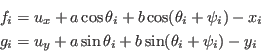
example consider the following functions:
variables. The procedure will choose the
bisected variables using, for example, the smear function. But in some
cases it may be interesting to guide the bisection: for example if we
know that subsets of the variables have a strong influence
on the extremal value of the
optimum function it may be interesting to indicate that as soon as the
smear function has led to bisecting one variable in a given subset it
may be good to bisect also the other variables in the subset. For
example consider the following functions:
where
 are unknowns and
  are given. Consider now the optimum function :
which has 24 unknowns. But clearly each subset
 has a strong influence on the minimum of . Hence if one of the
 is bisected it may be interesting to bisect also
 . This may be done by setting the flag
ALIAS_Guide_Bisection to 1
and using the
variables table:
for a problem with unknowns the variables table is an array of
size
. This may be done by setting the flag
ALIAS_Guide_Bisection to 1
and using the
variables table:
for a problem with unknowns the variables table is an array of
size  and a 1 in
  indicates that if the variable
is bisected then the variable
indicates that if the variable
is bisected then the variable  should be also bisected. In
ALIAS the variables table is implemented under the name
ALIAS_Bisecting_Table.
It is the responsibility of the user to
clear this array and update it as in the following example:
should be also bisected. In
ALIAS the variables table is implemented under the name
ALIAS_Bisecting_Table.
It is the responsibility of the user to
clear this array and update it as in the following example:
	Resize(ALIAS_Bisecting_Table,24,24);
	Clear(ALIAS_Bisecting_Table);
	ALIAS_Bisecting_Table(1,2)=1;
	ALIAS_Bisecting_Table(2,1)=1;
	ALIAS_Bisecting_Table(3,4)=1;
	ALIAS_Bisecting_Table(4,3)=1;
Consider the equation:
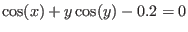 which defines a curve in the
  plane on which you want to
determine the closest point to the origin when
plane on which you want to
determine the closest point to the origin when  lie in the range
![$[-\pi,\pi]$](img277.png) . This leads to trying to
find the minimum of the function
. This leads to trying to
find the minimum of the function  under the constraint
.
under the constraint
.
The procedure for the interval evaluation of the 2 functions will be
written as:
INTERVAL_VECTOR IntervalTestFunction (int l1,int l2,INTERVAL_VECTOR & in)
// interval valued test function
{
INTERVAL x,y;
INTERVAL_VECTOR xx(2);

x=in(1);
y=in(2);
if(l1==1)
  xx(1)=Cos(x)+y*Sqr(Cos(y))-0.2;
if(l1<=2 && l2>=2)
  xx(2)=Sqr(x)+Sqr(y);
  return xx;
}
while the main program may be written as:
int main()
{
int Iterations, Dimension,Dimension_Eq,Num,i,j,precision;
double Accuracy,Accuracy_Variable;
INTERVAL_MATRIX SolutionList(2,2);
INTERVAL_VECTOR TestDomain(2),F(2),P(2),H(2);
INTEGER_VECTOR Type(2);
INTERVAL Optimum;
REAL pi;

pi=Constant::Pi;

Dimension_Eq=2;Dimension=2;
TestDomain(1)=INTERVAL(-pi,pi);TestDomain(2)=INTERVAL(-pi,pi);

cerr << "Number of iteration = "; cin >> Iterations;
cerr << "Accuracy on Function = "; cin >> Accuracy;

Type(1)=0;Type(2)=-2;
Accuracy=0;

Num=Minimize_Maximize(Dimension,Dimension_Eq,Type,
       IntervalTestFunction,TestDomain,Iterations,Accuracy_Variable,
       Accuracy,0,Optimum,SolutionList);
if(Num<0)
  {
    cout << "The procedure has failed, error code:"<<Num<<endl;
    return 0;
  }
cout<<"Optimum:"<<Optimum<<" obtained at"<<endl;
for(i=1;i<=Num;i++)
  {
    cout << "x=" << SolutionList(i,1) <<endl;
    cout << "y=" << SolutionList(i,2) <<endl;
  }
  return 0;
}
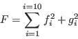
The Minimize_Maximize
and Minimize_Maximize_Gradient procedures will return the
same numerical results but the number of boxes will change.
The
results obtained for a full bisection,
the MAX_MIDDLE_FUNCTION_ORDER
and according to the accuracy epsilonf and the storage mode
(either direct (DSM) or reverse (RSM), see section 2.3.1.2) are
presented in the
following table (the number of boxes for the
Minimize_Maximize_Gradient procedure is indicated in
parenthesis):
| epsilonf |
Minimum |
 |
 |
boxes |
|
0.01, DSM |
[1.12195667, 1.12195667] |
[-0.944932,-0.4786] |
[-0.944932,-0.4786] |
76 (36) |
|
0.01, RSM |
[1.12195667, 1.12195667] |
[-0.944932,-0.4786] |
[-0.944932,-0.4786] |
59 (37) |
|
0.001, DSM |
[1.1401661,1.1401661] |
[-0.954903,-0.477835] |
[-0.954903,-0.477835] |
201 (75) |
|
0.001, RSM |
[1.1401661,1.1401661] |
[-0.954903,-0.477835] |
[-0.954903,-0.477835] |
148 (67) |
|
0.000001, DSM |
[1.14223267,1.14223267] |
[-0.957596,-0.474596] |
[-0.957596,-0.474596] |
5031 (2041) |
|
0.000001, RSM |
[1.14223267,1.14223267] |
[-0.957596,-0.474596] |
[-0.957596,-0.474596] |
4590 (2164) |
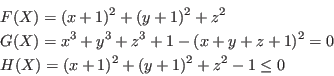
Consider the problem of finding the coordinates  of a point
that lie on the surface
of a point
that lie on the surface
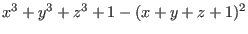 , is inside the
sphere centered at (-1,-1,0) of radius 1 and is the closest possible
to the center of this sphere, with the constraint that
lie in the range [-2,2]. Thus we have:
, is inside the
sphere centered at (-1,-1,0) of radius 1 and is the closest possible
to the center of this sphere, with the constraint that
lie in the range [-2,2]. Thus we have:
With epsilonf=0.0001 we find out that the point is located at
at (-0.747,-0.747,0.086059) which is well inside the sphere and that
the minimal distance is 0.13529.
We may also compute the minimal distance not to a point but to a line segment,
for example
defined by
![$x \in [0.9,1.1]$](img764.png) ,
,  ,
,  . In that case the optimum
function in the
evaluation procedure may be defined as:
. In that case the optimum
function in the
evaluation procedure may be defined as:
Sqr(x+INTERVAL(0.9,1.1))+Sqr(y+1)+Sqr(z)
and with epsilonf=0.0001 the algorithm will return that the
minimal distance lie in the range [0.0907,0.1925].


 Next: Continuation for one dimensional
Up: ALIAS-C++
Previous: Linear algebra
Next: Continuation for one dimensional
Up: ALIAS-C++
Previous: Linear algebra