 (for the MathML variant,
see here).
(for the MathML variant,
see here).
This page contains the description of the following commands
\a,
\AA,
\aa,
\abarnodeconnect,
\above,
\abovedisplayshortskip,
\abovedisplayskip,
\abovewithdelims,
\accent,
\accentset,
\active,
\acute,
\AddAttToIndex,
\AddAttToDocument,
\AddAttToCurrent,
\AddAttToLast,
\@addnl,
\addtocounter,
\addtolength,
\addto@hook,
\@addtoreset,
\addvspace,
\adjdemerits,
\advance,
\AE,
\ae,
\afterassignment,
\@afterelsefi,
\@afterfi,
\aftergroup,
\aleph,
\allowbreak,
\alph,
\Alph,
\@alph,
\@Alph,
\alpha,
\amalg,
\amp,
\anchor,
\anchorlabel,
\and,
\AND,
\angle,
\anodeconnect,
\anodecurve,
\aparaitre,
\apostrophe,
\ApplyFunction,
\approx,
\approxeq,
\arabic,
\@arabic,
\arc,
\arccos,
\arcsin,
\arctan,
\arg,
\arraycolsep,
\arrayrulewidth,
\arrowvert,
\Arrowvert,
\ast,
\asymp,
\AtBeginDocument,
\AtEndDocument,
\AtEndOfClass,
\AtEndOfPackage,
\atop,
\atopwithdelims,
and environments
abstract,
align,
alignat,
aligned,
array,
or concepts
accent.
The \a command can be used to put accents in a tabbing environment. This environment is not implemented in Tralics. If you say \a', it is the same as if you had said \'. The following shows some errors provoked by the misuses of this command.
>  \a{}e
Error signaled at line 1:
wanted a single token as argument to \a.
>  \a{foo}
Error signaled at line 2:
wanted a single token as argument to \a.
>  \a\foo
Error signaled at line 3:
Bad syntax of \a, argument not a character \foo.
>  \a+
Error signaled at line 4:
Bad syntax of \a, argument is {Character + of catcode 12}.
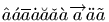
The \aa command translates into å or å. It is valid in math mode also. See the latin supplement characters.
The \AA command translates into Å or Å. This character is valid in math mode also. See the latin supplement characters.
The command \abarnodeconnect[d]{F}{T} connects nodes F and T using a bar with an arrow, with depth d.
A tree is defined by some nodes and connectors. Each node has a name, whose scope is limited to the current page (Tralics does no validity test for the names). A connector can be attached to the top, bottom, left or right of a node (abbreviation is one character of tblr), or a corner (two letter, one of tb followed by one of lr). In some cases a dimension is needed (this is a sequence of characters that can be interpreted as a dimension by the XML post-processor). All commands for the pst-tree package produce an element that has the same name as the command (\nodepoint is an exception). Elements associated to connectors are empty. See the pst-tree documentation for the meaning of all the parameters, that are not tested by Tralics.
\node{a}{Value of node A}
\nodepoint{b} \nodepoint{c}[3pt]\nodepoint{d}[4pt][5pt]
\nodeconnect{a}{b}
\nodeconnect[tl]{a}[r]{c}
\anodeconnect{a}{b}
\anodeconnect[tl]{a}[r]{c}
\barnodeconnect[3pt]{a}{d}
\nodecurve{a}{b}{2pt} ?
\nodecurve[l]{a}[r]{b}{2pt}[3pt]
\nodetriangle{a}{b}
\nodebox{a}
\nodeoval{a}
\nodecircle[3pt]{a}
<node name='a'>Value of node A</node>
<node name='b'/>
<node xpos='3pt' name='c'/><node ypos='5pt' xpos='4pt' name='d'/>
<nodeconnect nameA='a' nameB='b' posA='b' posB='t'/>
<nodeconnect nameA='a' nameB='c' posA='tl' posB='r'/>
<anodeconnect nameA='a' nameB='b' posA='b' posB='t'/>
<anodeconnect nameA='a' nameB='c' posA='tl' posB='r'/>
<barnodeconnect nameA='a' nameB='d' depth='3pt'/>
<nodecurve nameA='a' nameB='b' posA='b' posB='t' depthB='2pt' depthA='2pt'/>?
<nodecurve nameA='a' nameB='b' posA='l' posB='r' depthB='3pt' depthA='2pt'/>
<nodetriangle nameB='b' nameA='a'/>
<nodebox nameA='a'/>
<nodeoval nameA='a'/>
<nodecircle nameA='a' depth='3pt'/>
The \above command is a TeX primitive that should not be used. Instead of aa \above1pt bb you should use \genfrac{}{}{1pt}{}{aa}{bb}. Note that the dimension is an argument in the case of \genfrac, while Tralics uses an ad-hoc strategy to find it in the other case (two characters are read after digits or decimal point). In particular \dimen0 is valid in the case of \genfrac but not in the case of \above. See \genfrac and \over.
You can say \abovedisplayshortskip=10pt plus 2pt minus 3pt. The \abovedisplayshortskip register contains a skip value that TeX puts before a short display. The value is unused by Tralics. (See scanglue for details of argument scanning). (See \predisplaysize for further details).
You can say \abovedisplayskip=10pt plus 2pt minus 3pt. The \abovedisplayskip register contains a skip value that TeX puts before a display. The value is unused by Tralics. (See scanglue for details of argument scanning). (See \predisplaysize for further details).
The \abovewithdelims command is a TeX primitive that should not be used. Instead of aa \abovewithdelims()1pt bb you should use \genfrac(){1pt}{}{aa}{bb}. See \genfrac and \over. See \above above.
The abstract environment is defined as \newenvironment{abstract}{}{} in versions up to 2.3 for compatibility reasons. It is now a user-defined environment for the Raweb only. It is undefined otherwise.
This command is unimplemented; see here for details.
There are different ways to put an accent over a letter. You can say \accent, but this is a TeX primitive not implemented in Tralics.
You can say $\hat{a} \acute{a} \bar{a} \dot{a} \breve{a} \check{a} \grave{a}
\vec{a} \ddot{a} \tilde{a}$, but these commands work only in math mode,
they produce characters like this image
(for the MathML variant,
see here).
You can say éîÀ, but this works only if the character exists in the current input encoding.
You can say \`e \'e \^e \"e \~a \.e \=e
(this gives  ), or
\c c, \H o, \C o, \"o, \k a, \b b, \d a, \u a, \f a, \v a, \T e, \r a, \D a, \h a, \V e.
(this gives
), or
\c c, \H o, \C o, \"o, \k a, \b b, \d a, \u a, \f a, \v a, \T e, \r a, \D a, \h a, \V e.
(this gives  ).
\k is not in Lamport, but is defined in t1enc.def. The same is
true for \r. The \f and \C commands
are defined by the t2aenc.def file. The \T command (tilde below),
\V (circonflex below), \D (circle below),
\h (hook) are defined only by Tralics.
The \t command is not yet implemented. Not all combinations
exist, see each individual command for what letters are accepted.
).
\k is not in Lamport, but is defined in t1enc.def. The same is
true for \r. The \f and \C commands
are defined by the t2aenc.def file. The \T command (tilde below),
\V (circonflex below), \D (circle below),
\h (hook) are defined only by Tralics.
The \t command is not yet implemented. Not all combinations
exist, see each individual command for what letters are accepted.
Double accents: in general, you can only put an accent over a letter.
In some cases you can put an accent over an accented character. Here are some
examples:
\={\.a} \={\"a}, \"{\'u} \"{\`u} \"{\v u} \c{\'c} \c{\u e}
\d{\. s} \'{\^e}. This gives
 .
.
Strange accents. If you say
\=\ae \'\ae \'\aa \'\o \'\i , then you will see
 . The first element in the
list can also be entered as ^^^^01e2, because it corresponds to
Unicode character U+1E2. Note that this character is as valid as, say, a comma,
hence can be used in math mode. Translation is
<mi>Ǣ</mi>, as is the case for all
non-ascii characters.
. The first element in the
list can also be entered as ^^^^01e2, because it corresponds to
Unicode character U+1E2. Note that this character is as valid as, say, a comma,
hence can be used in math mode. Translation is
<mi>Ǣ</mi>, as is the case for all
non-ascii characters.
Since version 2.12, Tralics accepts to put an accent on any (7bit ASCII) letter. For instance, \D e produces the following two characters: e̥ that should render as e̥. In the following example, all characters but the last in the list translate into a single Unicode character, the last one uses a combination.
\def\acclist#1#2{\def\theacc{#1}\let\next\oneacc\next#2\relax}
\def\Relax{\relax}
\def\oneacc#1{%
\ifx#1\relax\let\next\relax\else\theacc#1 \fi
\next}

\acclist\`{AEIOUNWYaeiounwyx}\par
\acclist\'{AEIOUYCLNRSZGKMPW\AE\AA\O\ae\aa\o aeiouyclnrszgkmpwv}\par
\acclist\^{AEIOUCGHJSWYZaeioucghjswyz}\par
\acclist\~{ANOUIVEYioanoioveyw}\par
\acclist\"{AEIOUYHWXaeiouyhwxtz}\par
\acclist\H{OUoue}\par
\acclist\r{AUauwye}\par
\acclist\v{CDELNRSTZAIUGKHcdelnrstzaiugkhjx}\par
\acclist\u{AEGIOUaegioux}\par
\acclist\={AEHIOTUYG\AE\ae aehiotuyg}\par
\acclist\.{ABCDEFGHILMNOPRSTWXYZabcdeghlmnoprstuvwzyzq}\par
\acclist\c{CGKLNRSTEDHcgklnrstedhb}\par
\acclist\k{AEIOUaeioub}\par
\acclist\D{AEIOURaeioury}\par
\acclist\b{BDKLNRTZbdklnrtzhe}\par
\acclist\d{BDHKLMNRSTVWZAEIOUYbdhklmnrstvwzaeiouyc}\par
\acclist\f{AEIOURaeiourx}\par
\acclist\T{EIUeiuo}\par
\acclist\V{DELNTUdelntua}\par
\acclist\D{Aae}\par
\acclist\h{AEIOUYaeiouyx}
The tipa/tipx package defines some double accents. Commands like \textacutemacron produce a macron and an acute accent over the letter. Since version 2.12, you can use \'=e as a short-hand. Note that \'{\=e} produces character U+1E17 and \'{\=e} gives an error. You can put an acute accent over any character via the construct \=e^^^^0301. The Unicode standard says that this should be the same as e^^^^0304^^^^0301, but this looks ugly in some cases; for this reason, an under caron is used. You get a̖ a̖ ạ̀ ạ̀ à̱ à e̗ e̗ é̱ é̱ é o̭ o̭ ộ ộ ô ṵ ṵ ụ͂ ụ͂ ũ a̤ a̤ ä ę ę e̋ o̥ u̥ o̱̊ o̱̊ o̊ u̬ u̬ ú̬ á̬ ǔ a̯ a̯ ă̠ ă̠ ă e̱ e̱ ē ọ ẹ ọ́ ọ́ a̐ u̇ ‿au a͡e g͡b via the following input:
\`*a \textsubgrave{a} \`.a \textgravedot{a} \textgravemacron{a} \`a
\'*e \textsubacute{e} \'=e \textacutemacron{e} \'e
\^*o \textsubcircum{o} \^.o \textcircumdot{o} \^o
\~*u \textsubtilde{u} \~.u \texttildedot{u} \~u
\"*a \textsubumlaut{a} \"a
\H*e \textdoublegrave{e} \H e
\r*o \textsubring{u} \r=o \textringmacron{o} \r o
\v*u \textsubwedge{u} \v'u \textacutewedge{a} \v u
\u*a \textsubarch{a}  \u=a \textbrevemacron{a} \u a
\=*e \textsubbar{e} \=e
\.*o \textsubdot{e} \.'o \textdotacute{o} \textdotbreve{a} \.u
\t*au \t ae \texttoptiebar gb
The tipa package provides some additional accents; they are obtained via a construction of the form \|m{t}. This needs redefinition of the \| command (that produces a double vertical bar in math mode). This redefinition is not done if the package is loaded in safe mode. You can redefine the command as shown below; you can also use the long name, here \textseagull. The symbols t̪ t̪ d̺ d̺ o̹ o̹ o̜ o̜ g̑ g̑ ɔ̟ o̟ e̞ e̞ ɛ̝ e̝ u̘ u̘ ə̙ e̙ e̽ e̽ k̫ k̫ t̼ t̼ are produced by the following input:
{\makeatletter \global\let\|\@omniaccent}
\textsubbridge{t} \|[t      \textinvsubbridge{d} \|]d
\textsubrhalfring{o} \|)o   \textsublhalfring{o} \|(o
\textroundcap{g} \|c{g}     \textsubplus{\textopeno} \|+o
\textlowering{e} \|`e       \textraising{\textepsilon} \|'e
\textadvancing{u} \|<u      \textretracting{\textschwa} \|>e
\textovercross{e} \|x{e}    \textsubw{k} \|w{k}
\textseagull{t} \|m{t}
The tipa package provides \super as an abbreviation for \textsuperscript. A superscript H can also be given directly using Unicode character U+02B0. Here are some examples, using both alternatives ph = pʰ kw=kʷ tj=tʲ dɣ=dˠ dʕ=dˁ dn dl=dˡ, and this is the source.
p\super h = p^^^^02b0
k\super w=k^^^^02b7 t\super j=t^^^^02b2  d\super\textgamma=d^^^^02e0
d\super{\textrevglotstop}=d^^^^02c1
d\super n d\super l=d^^^^02e1
The next example uses the tipa package
\textpolhook{e} \textrevpolhook{o} \textvbaraccent{a}
\textdoublevbaraccent{a} \textsubsquare{n}
\textsyllabic{m} \textsuperimposetilde{t} t\textcorner{} t\textopencorner{}
\textschwa\textrhoticity{} b\textceltpal{} k\textlptr{} k\textrptr{}

\spreadlips{s} \overbridge{v} \bibridge{n} \subdoublebar{t}
\subdoublevert{f} \subcorner{v} \whistle{s} \sliding\texttheta s
\crtilde{m}  \doubletilde{s} \sublptr{J} \subrptr{J}

\textglotstop, \textglotstopvari, \textglotstopvarii, \textglotstopvariii,
\textraiseglotstop, \textbarglotstop, \textinvglotstop,
 \textcrinvglotstop, \textctinvglotstop,
\textturnglotstop, \textrevglotstop, \textbarrevglotstop

\textpipe, \textpipevar, \textdoublebarpipe, \textdoublebarpipevar,
\textdoublebarslash, \textdoublepipevar

x\textprimstress y x\textsecstress y
x\textlengthmark y x\texthalflength y
x\textbottomtiebar y  x\textdownstep y
x\textupstep y \textdownstep \textupstep \textglobfall \textglobrise
\textspleftarrow \textdownfullarrow \textupfullarrow
\textsubrightarrow \textsubdoublearrow

\tone{55}\tone{44}\tone{33}\tone{22}\tone{11}
\tone{51}\tone{15}\tone{45}\tone{12}\tone{454}

\texthighrise{a} \textlowrise{a} \textrisefall{a} \textfallrise{a}
Translation
ę o̧ a̍ a̎ n̻ m̩ t̴ t˺ t˹ ə˞ bˊ k< k>
s͍ v͆ n̪͆ t͇ f͈ v͉ s͎ θ͢s m͊ s͌ J͔ J͕
ʔ, ʔ, ʔ, ʔ, ʔ, ʡ, ʖ, ʖ, ʖ, ʖ, ʕ, ʢ
ǀ, ǀ, ǂ, ǂ, ≠, ǁ, !
xˈy xˌy x:y xˑy x‿y xAy xAy AA↘↗A↓↑AA
˥˦˧˨˩
ā́ à̄ à́̀ á̀́
Like \underaccent, but the accent is above. This is valid in math mode only, translation of \accentset xy is <mover accent='true'><mi>y</mi> <mi>x</mi></mover> (for an example, see here).
This command is made equal to 13 via \chardef. Use it only when a number is required. Use it in cases like \catcode~=\active (for an example, see \aftergroup).
The \acute command puts an acute accent over a kernel. It works only in math mode (in text mode, you should use the \' command). The math accents recognized by Tralics are the following
$\acute{x} \bar{x} \breve{x} \check{x}
\ddddot{x} \dddot{x} \ddot{x} \dot{x}
\grave{x} \hat{x} \mathring{x} \tilde{x}
\vec{x} \widehat{xyz} \widetilde{xyz}$
The XML result is
<formula type='inline'> <math xmlns='http://www.w3.org/1998/Math/MathML'> <mrow> <mover accent='true'><mi>x</mi> <mo>´</mo></mover> <mover accent='true'><mi>x</mi> <mo>‾</mo></mover> <mover accent='true'><mi>x</mi> <mo>˘</mo></mover> <mover accent='true'><mi>x</mi> <mo>ˇ</mo></mover> <mover accent='true'><mi>x</mi> <mo>⃜</mo></mover> <mover accent='true'><mi>x</mi> <mo>⃛</mo></mover> <mover accent='true'><mi>x</mi> <mo>¨</mo></mover> <mover accent='true'><mi>x</mi> <mo>˙</mo></mover> <mover accent='true'><mi>x</mi> <mo>`</mo></mover> <mover accent='true'><mi>x</mi> <mo>^</mo></mover> <mover accent='true'><mi>x</mi> <mo>˚</mo></mover> <mover accent='true'><mi>x</mi> <mo>˜</mo></mover> <mover accent='true'><mi>x</mi> <mo>→</mo></mover> <mover accent='true'><mrow><mi>x</mi><mi>y</mi><mi>z</mi></mrow> <mo>^</mo></mover> <mover accent='true'><mrow><mi>x</mi><mi>y</mi><mi>z</mi></mrow> <mo>˜</mo></mover> </mrow> </math> </formula>
All these commands are listed in Table 8.12 of the Latex Companion 2.
Preview:  (see also here).
Note that \widehat and \widetilde are not wide in the current implementation.
(see also here).
Note that \widehat and \widetilde are not wide in the current implementation.
Other constructs look like accents, but use large or extensible symbols.
$%
\widetilde{abc} \widehat{abc} \overleftarrow{abc} \overrightarrow{abc}
\overline{abc} \underline{abc} \overbrace{abc} \underbrace{abc}
\underleftarrow{abc} \underrightarrow{abc}
$
The XML result is
<formula type='inline'><math xmlns='http://www.w3.org/1998/Math/MathML'> <mrow><mover accent='true'><mrow><mi>a</mi><mi>b</mi><mi>c</mi></mrow> <mo>˜</mo></mover> <mover accent='true'><mrow><mi>a</mi><mi>b</mi><mi>c</mi></mrow> <mo>^</mo></mover> <mover accent='true'><mrow><mi>a</mi><mi>b</mi><mi>c</mi></mrow> <mo>←</mo></mover> <mover accent='true'><mrow><mi>a</mi><mi>b</mi><mi>c</mi></mrow> <mo>→</mo></mover> <mover accent='true'><mrow><mi>a</mi><mi>b</mi><mi>c</mi></mrow> <mo>‾</mo></mover> <munder accentunder='true'><mrow><mi>a</mi><mi>b</mi><mi>c</mi></mrow> <mo>_</mo></munder> <mover accent='true'><mrow><mi>a</mi><mi>b</mi><mi>c</mi></mrow> <mo>⏞</mo></mover> <munder accentunder='true'><mrow><mi>a</mi><mi>b</mi><mi>c</mi></mrow> <mo>⏟</mo></munder> <munder accentunder='true'><mrow><mi>a</mi><mi>b</mi><mi>c</mi></mrow> <mo>←</mo></munder> <munder accentunder='true'><mrow><mi>a</mi><mi>b</mi><mi>c</mi></mrow> <mo>→</mo></munder> </mrow></math></formula>
These commands are listed in Table 8.12 of the
Latex Companion.
Preview: 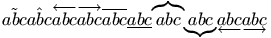
Other constructs:
$\stackrel{j}{\longrightarrow} \overset{*}{X} \underset{*}{X}
\sqrt{abc} \sqrt[n]{abc} \root n \of{abc}
\frac{abc}{xyz} \dfrac{abc}{xyz}$
The XML result is
<formula type='inline'><math xmlns='http://www.w3.org/1998/Math/MathML'>
<mrow>
<mover><mo>⟶</mo> <mi>j</mi></mover>
<mover><mi>X</mi> <mo>*</mo></mover>
<munder><mi>X</mi> <mo>*</mo></munder>
<msqrt><mrow><mi>a</mi><mi>b</mi><mi>c</mi></mrow></msqrt>
<mroot><mrow><mi>a</mi><mi>b</mi><mi>c</mi></mrow> <mi>n</mi></mroot>
<mroot><mrow><mi>a</mi><mi>b</mi><mi>c</mi></mrow> <mi>n</mi></mroot>
<mfrac><mrow><mi>a</mi><mi>b</mi><mi>c</mi></mrow>
<mrow><mi>x</mi><mi>y</mi><mi>z</mi></mrow>
</mfrac>
<mstyle scriptlevel='0' displaystyle='true'>
<mfrac>
<mrow><mi>a</mi><mi>b</mi><mi>c</mi></mrow>
<mrow><mi>x</mi><mi>y</mi><mi>z</mi></mrow>
</mfrac>
</mstyle>
</mrow>
</math></formula>
Preview: 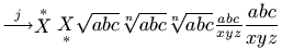
If you say \AddAttToIndex[idx-name]{att-name}{att-val}, this will add an attribute pair to the index named idx-name, of the form att-name='att-val'; see \index for an example. An alternate name is \addattributetoindex.
The \AddAttToDocument command takes two arguments A and B. It adds A='B' to the attribute list of the document element. It is the same as \XMLaddatt[1]{A}{B}. Alternate names are \addattributetodocument or \addattributestodocument. See \XMLaddatt.
The \AddAttToCurrent command takes two arguments A and B. It adds A='B' to the attribute list of the current element. See the xmlelement environment. \AddAttToCurrrent{X}{Y} is the same as \XMLaddatt{X}{Y}. See \XMLaddatt.
The \AddAttToLast command takes two arguments A and B. It adds A='B' to the attribute list of the element created latest. See the xmlelement environment. Note that \AddAttToLast{X}{Y} is the same as \XMLaddatt[\the\XMLlastid]{X}{Y}. See \XMLaddatt.
This command inserts a new line character in the XML tree.
The \addtocounter command takes two arguments, a counter and a value (see counters in latex). It increments the value of the counter by the given amount. Modification is always global. If you say \addtocounter{foo}{10} the result is as if you had said \global\advance\c@foo 10\relax (see scanint for details of how \advance reads a number).
If the calc package is loaded, the result is as if you had said \calc{\global\advance\c@foo} {10}. Here 10 could be replaced by 2*5. See the calc package for an example. The example here shows the expansion of the command.
> \newcounter{foo}
> \toks0=\expandafter{\addtocounter{foo}{25}}
> \showthe\toks0
\show: \global \advance \c@foo 25\relax
Instead of \addtolength\foo{10cm}, you can say \advance\foo 10cm\relax. The result is the same. (see scandimen for details of how a dimension or a glue is scanned; if the argument, here \foo, is not a reference to something that reads an integer, a dimension, a glue or a muglue, a strange error might be signaled).
If the calc package is loaded, the input is handled as \calc{\advance\cfoo}{10cm}. See the calc package for an example.
Saying \addto@hook\foo{bar} has as effect to add the token list bar at the end of the hook \foo (a reference to a token list register). See also \@cons.
Saying \@addtoreset{footnote}{chapter} has as effect to reset the footnote counter whenever the chapter counter is incremented by \stepcounter. Note that before version 2.13, Tralics did not use nor modify these two counters. Currently, these counters are incremented whenever a new chapter or footnote is started, and used by \thechapter or \thefootnote when computing the id-text attribute associated to the div or note element.
The \addvspace command takes an argument; it is defined in LaTeX as follows: outside vertical mode, it provokes an error; inside a minipage environment it does nothing. Otherwise, let A the value of \lastskip and B be the value of the argument, converted to a dimension. It A is zero, then a \vskip of value B is added to the main vertical list. If A is less than B, two \vskips are added: minus A, then B. If A and B are negative, nothing is done. If B is negative, and A is positive, two \vskips are added: minus A, and the sum of A and B.
Note that \vspace 10cm is the same as \vskip10cm\vskip0pt, so that, after a \vspace \lastskip returns 0.
This command is not implemented, mainly because \lastskip does not work.
When you say \adjdemerits=93, then TeX will use 93 as additional demerits for a line visually incompatible with the previous one. Unused by Tralics. (See scanint for details of argument scanning).
If you say \global\advance\count0 by 1, the value of \count0 is globally incremented by 1. The keyword by is optional. Instead of \count0 you can put any variable that remembers an integer, a dimension, a glue, or a muglue; after the optional by an integer (a dimension, a glue, or a muglue, depending on the case) is scanned. Note that you cannot put, after \advance, a command that reads a restricted integer (for instance, \catcode, and such).
The \ae command generates the æ character, this is also æ. This character is valid in math mode also. For details, see the latin supplement characters.
The \AE command generates the Æ character, this is also Æ. This character is valid in math mode also. For details, see the latin supplement characters.
When you say \afterassignment\foo, the token \foo is saved somewhere, and used just after the next assignment. Unlike \aftergroup, this token is not saved on the stack, so that in the case of two consecutive \afterassignment, the first one is lost. Example:
\def\foo{123}
\afterassignment\foo\setbox0=\hbox{4}
In this case, the assignment is considered complete when the open brace is read after \hbox. Thus box0 will contain 1234. A typical use of \afterassignment is given here.
\makeatletter
\def\openup{\afterassignment\@penup\dimen@=}
\def\@penup{\advance\lineskip\dimen@
  \advance\baselineskip\dimen@
  \advance\lineskiplimit\dimen@}
\makeatother
\openup1234pt
In LaTeX, you would say:
\def\Openup#1{\addtolength{\lineskip}{#1}
  \addtolength{\baselineskip}{#1}
  \addtolength{\lineskiplimit}{#1}}
\Openup{1234pt}
but this definition is less efficient. Of course, \Openup could read an argument, put the result in \dimen@, and call \advance. The reason for \afterassignment is that the argument of \openup is not delimited by braces: the scandimen routine reads as many tokens as needed. The commands \vglue, \hglue, and \magnification use this same trick.
Other example. This is \settabs, from plain, where some macros have been renamed.
\def\settabs{... \futurelet\nexttoken\settab@I}
\def\settab@I{\ifx\nexttoken\+%
  \def\nextcmd{\afterassignment\settab@II\let\nextcmd}%
  \else\let\nextcmd\s@tcols\fi
  \let\nexttoken\relax
  \nextcmd}
\def\settab@II{\let\nextcmd\relax action}
\def\s@tcols#1\columns{action}
The idea is the following: \settabs is either followed by a sample line (that starts with \+), or something like 25\columns. The effect of \futurelet \nexttoken \settab@I is to read the next token (\+ or 2), put it in \nexttoken, push it back in the input stream, and call \settab@I. This command tests whether the token is \+ or not, it sets \nextcmd, kills \netxttoken, and calls \nextcmd. When you say \settabs 25\columns, the \s@tcols command is called with a delimited argument. Otherwise, we see the \afterassignment\settab@II, followed by \let\nextcmd. This is an assignment: it puts in \nextcmd the token that follows (the \+) then calls \settab@II, that kills \nextcmd and does some action.
There are two problems here: check whether the next token is \+, and read it. It is not possible to read this token as an argument because the token is \outer. On the other hand, both \nextcmd and \nexttoken have to be killed (made equivalent to \relax) because it is unwise to have useless \outer tokens. In the TeXbook, Knuth uses one token \next instead of two tokens \nextcmd and \nexttoken, why?
Other example (from the LaTeX source)
\def\restore@protect{\let\protect\@@protect}
\def\protected@edef{%
   \let\@@protect\protect
   \let\protect\@unexpandable@protect
   \afterassignment\restore@protect
   \edef
}
Hence \protected@edef\foo{\bar} is the same as
\let\copy@of@protect \protect
\let\protect \a@protect@designed@for@edef
\edef\foo{\bar}
\let\protect \copy@of@protect
Assume that you want to use conditionnaly a command, you can do this \ifnum\count0=0 \foo\else\bar\fi. This works only if the command takes no argument, otherwise you must use something more complicated like \ifnum\count0=0 \expandafter\foo\else\expandafter\bar\fi. The situation is worse if the command takes two arguments, one before and one after the conditional. The two commands \@afterelsefi and \@afterfi can be placed before \foo and \bar, the effect is to read all relevant tokens (until \else or \fi), discard the unwanted ones (those between \else and \fi, if the condition is true), terminate the condition, and re-insert the tokens. Example
\def\xfoo#1#2{\def\testa{x#1#2}}
\def\yfoo#1#2{\def\testb{y#1#2}}
\def\test#1{\ifnum0=#1 \@afterelsefi\xfoo u \else\@afterfi\yfoo v\fi}
% run the test
\test0a \test1b
% check
\def\testA{xua}\def\testB{yvb}
\ifx\testa\testA\else\bad\fi
\ifx\testb\testB\else\bad\fi
When you say \aftergroup, a token is read, and pushed on the save stack. At the end of the group, the token is pushed back in the input stream. Example.
{\def\A{A}\def\B{B}\def\C{C}
{\def\A{AA}\def\B{BB}\def\C{CC}\aftergroup\A \aftergroup\B\C}}
The translation is CCAB.
In fact, \C expands to CC. After that the closing brace has as effect to unwind the stack: old definitions of \A, \B and \C are restored, and the tokens \A and \B are inserted in the stream. Elements are popped in the reverse order as they were pushed: \B is inserted first, and \A is restored last. Since \A is popped after \B it is the first token to be read again. This is what the transcript file says:
{end-group character}
+stack: after group \B
+stack: after group \A
+stack: restoring \C=macro:->C.
+stack: restoring \B=macro:->B.
+stack: restoring \A=macro:->A.
This is an example from the TeXbook, appendix D, instantiated with \n=5. It is equivalent to \edef\ast{*****}.
\countdef\n 3
\n=5
\begingroup\aftergroup\edef\aftergroup\asts\aftergroup{
\loop\ifnum\n>0 \aftergroup*\advance\n-1 \repeat
\aftergroup}\endgroup
As the transcript file below shows, the result is formed of the three tokens \edef\asts{, followed by N copies of *, followed by }. These things are gathered when \endgroup is seen. Since the \loop is local to the group, two quantities are restored: a command named \iterate and the counter.
+stack: after group {Character } of catcode 2}
+stack: after group {Character * of catcode 12}
+stack: after group {Character * of catcode 12}
+stack: after group {Character * of catcode 12}
+stack: after group {Character * of catcode 12}
+stack: restoring \count3=5.
+stack: after group {Character * of catcode 12}
+stack: killing \iterate
+stack: after group {Character { of catcode 1}
+stack: after group \asts
+stack: after group \edef
Other example (simplified version of \verb). Consider the following definitions
{\catcode`\^^M=\active % these lines must end with %
  \gdef\obeylines{\catcode`\^^M\active \let^^M\par}%
  \global\let^^M\par} % this is in case ^^M appears in a \write
\begingroup
  \obeylines%
  \gdef\VEE{\obeylines  \def^^M{\verbegroup \verberrorA}}%
\endgroup
\let\VBG\empty
\def\verbegroup{\global\let\VBG\empty\egroup}
This defines \obeylines, whose effect is to make the new line an active character, equivalent to \par. After that it defines \VEE whose effect is to make the newline character active, and its value is now \verbegroup\verberror. The effect of \verbegroup is to reset (globally) \VBG to empty, and terminate the current group. The other command signals an error. Consider now:
\def\sverb{\bgroup \VEE \tt \ssverb}
\def\ssverb#1{%
  \catcode`#1\active
  \lccode`\~`#1%
  \gdef\VBG{\verbegroup\verberrorB}%
  \aftergroup\VBG
  \lowercase{\let~\verbegroup}}%
When you say \sverb x y x the following happens. A group is opened, some commands are executed, and \ssverb is called, with argument x. (In LaTeX, some category codes are changed, including the space character; as a result, the space that follows the command is no more ignored, and can be used as delimiter. As a consequence, no letter can be a delimiter). The letter x is made active, and defined to be \verbegroup. Moreover \VBG is defined to some command and saved for after group.
Assume that, as in the example, x is seen, hence executed. The \verbegroup command kills \VBG and executes \egroup. This \egroup has some side effects: it restores the \catcode of x, the current font, and whatever is needed. The \VBG token inserted by \aftergroup has no effect.
Assume that we have defined \def\test#1{{#1}} and say \test{\sverb x y x}. Note that the \catcode of the second x does not change, so that this x does not behave as above. When the brace of \test is evaluated, the category code of x is restored, and \VBG is executed. It calls \verbegroup (hence terminates the group opened by \sverb), then signals an error.
Same example, with \def\test#1{#1} instead. It is likely that there is no other x on the line that contains \test{\sverb x y x}, so that the end-of-line character is active, and calls \verbegroup \verberrorA. Thus a different error is signaled. This is the log file for the second example, with some comments added.
\test#1->{#1}
#1<-\sverb x y x
{begin-group character}
+stack: level + 3 for brace entered on line 28
\sverb-> \bgroup \VEE \tt \ssverb
{begin-group character}
+stack: level + 4 for brace entered on line 28
\VEE->\obeylines \def ^^M{\verbegroup \verberrorA }
\obeylines->\catcode `\^^M\active \let ^^M\par
{\catcode}
+scanint for \catcode->13 % this is ASCII code of ^M
+scanint for \catcode->13 % this is \active
{changing \catcode13=5 into \catcode13=13}
{\let}
{\let ^^M \par}
{changing ^^M=\par}
{into ^^M=\par}
{\def}
{changing ^^M=\par}
{into ^^M=macro:->\verbegroup \verberrorA }
{\tt}
{font change \ttfamily}
\ssverb#1->\catcode `#1\active \lccode `\~`#1\gdef \VBG {\verbegroup \verberrorB }
\aftergroup \VBG \lowercase {\let ~\verbegroup }
#1<-x
{\catcode}
+scanint for \catcode->120 % this is ASCII code of x
+scanint for \catcode->13 % this is \active
{\lccode}
{changing \catcode120=11 into \catcode120=13}
+scanint for \lccode->126% this is ASCII code of ~
+scanint for \lccode->120% this is ASCII code of x
{changing \lccode126=0 into \lccode126=120}
{\gdef}
{globally changing \VBG=macro:->}
{into \VBG=macro:->\verbegroup \verberrorB }
{\aftergroup}
{\lowercase}
{\lowercase(a)->\let ~\verbegroup }
{\lowercase->\let x\verbegroup }
{\let}
{\let x \verbegroup}
{changing x=undefined}
{into x=macro:->\global \let \VBG \empty \egroup }
Character sequence:  y x.
{end-group character}% closing brace of \test
+stack: killing x.
+stack: after group \VBG
+stack: restoring \lccode126=0. % the \lccode of ~
+stack: restoring \catcode120=11. % the \catcode of x
{Text:  y x} % These are the chars affected by \tt, there are two spaces
+stack: restoring current font .
+stack: restoring ^^M=\par.
+stack: restoring \catcode13=5.
+stack: level - 4 for brace  from line 28
\VBG->\verbegroup \verberrorB
\verbegroup->\global \let \VBG \empty \egroup
{\global}
{\global\let}
{\let \VBG \empty}
{globally changing \VBG=macro:->\verbegroup \verberrorB }
{into \VBG=macro:->}
{end-group character}
+stack: level - 3 for brace for brace from line 28
% this is followed by: Undefined command \verberrorB
The \aleph command is valid only in math mode.
It generates a miscellaneous symbol (Hebrew letter aleph):
<mo>ℵ</mo> (Unicode U+2135, ℵ),
that renders like
 .
See description of the
\ldots command.
.
See description of the
\ldots command.
The align environment (provided by the amsmath package) is used for two or more equations when vertical alignment is desired at n points (one in the example below). \begin{align} X&Y \end{align} is equivalent to $$\begin{array}{rl} X&Y \end{array}$$. (equation number does not work well in version 2.13). There are variants: flalign, alignat, xalignat and xxalignat. The last two environments are considered obsolete by amsmath. The three last environments take an optional argument (ignored by Tralics), the value of n. Note that Tralics assumes n=5, so that if you use more than ten columns, they will lack an alignment attribute. There are unnumbered variants align*, etc. The xxalignat environment occupies the whole width of the page, there is no place for an equation number, so is always unnumbered, and has no starred version (in Tralics all these environments behave the same). Example
\begin{align}
x^2+y^2&=1\\ x&=\sqrt{1-y^2}
\end{align}
Translation
<formula type='display'>
 <math mode='display' xmlns='http://www.w3.org/1998/Math/MathML'>
  <mtable displaystyle='true'>
   <mtr>
    <mtd columnalign='right'>
     <mrow><msup><mi>x</mi> <mn>2</mn> </msup>
        <mo>+</mo><msup><mi>y</mi> <mn>2</mn> </msup>
     </mrow>
    </mtd>
    <mtd columnalign='left'><mrow><mo>=</mo><mn>1</mn></mrow></mtd>
   </mtr>
   <mtr>
    <mtd columnalign='right'><mi>x</mi></mtd>
    <mtd columnalign='left'>
     <mrow><mo>=</mo><msqrt><mrow><mn>1</mn><mo>-</mo><msup><mi>y</mi>
        <mn>2</mn> </msup></mrow></msqrt>
     </mrow>
    </mtd>
   </mtr>
  </mtable>
 </math>
</formula>
Preview: 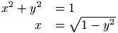 .
(see also here).
.
(see also here).
The aligned environment produces a display table (as align), a table that has an attribute that says this is a display table, and each cell is typeset in display style. Cells are alternatively right and left aligned. This environment must be used in a math formula. There is an optional argument that indicates vertical aligned (currently ignored by Tralics). Example
\begin{equation}
\begin{aligned}[x]
x^2+y^2&=1& 1&=X^2+Y^2\\
x&=0.01&0.001=X
\end{aligned}
\end{equation}
Translation
<formula id-text='3' id='uid3' type='display'>
 <math mode='display' xmlns='http://www.w3.org/1998/Math/MathML'>
  <mtable displaystyle='true'>
   <mtr>
    <mtd columnalign='right'>
      <mrow><msup><mi>x</mi> <mn>2</mn> </msup><mo>+</mo><msup><mi>y</mi>
            <mn>2</mn> </msup></mrow></mtd>
    <mtd columnalign='left'><mrow><mo>=</mo><mn>1</mn></mrow></mtd>
    <mtd columnalign='right'><mn>1</mn></mtd>
    <mtd columnalign='left'>
       <mrow><mo>=</mo><msup><mi>X</mi> <mn>2</mn> </msup><mo>+</mo><msup>
            <mi>Y</mi> <mn>2</mn> </msup></mrow></mtd>
   </mtr>
   <mtr>
    <mtd columnalign='right'><mi>x</mi></mtd>
    <mtd columnalign='left'><mrow><mo>=</mo><mn>0</mn><mo>.</mo><mn>01</mn></mrow></mtd>
    <mtd columnalign='right'>
      <mrow><mn>0</mn><mo>.</mo><mn>001</mn><mo>=</mo><mi>X</mi></mrow></mtd>
   </mtr>
  </mtable>
 </math>
</formula>
Preview: 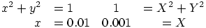 .
(see also here).
.
(see also here).
The translation of \allowbreak is <allowbreak/> since version 2.9.4. In previous versions, the command was ignored.
The \Alph command takes as argument a counter (see counters in latex), and typesets its value as a uppercase letter. The value of the counter has to be between 1 and 26. See example below.
The expansion of \Alph{foo} is \@Alph\c@foo and \@Alph calls scanint in order to get a number. The expansion is a letter (of category code 11).
The \alph command takes as argument a counter (see counters in latex), and typesets its value as a lower case letter. The value of the counter has to be between 1 and 26.
The expansion of \alph{foo} is \@alph\c@foo and \@alph calls scanint in order to get a number. The expansion is a letter (of \catcode 11).
In the example that follows, we show different ways to typeset a counter.
We put \fnsymbol in a math formula and outside it; the
documentation says: may be used only in math mode
but the code says
\ensuremath{...}.
\def\showcounter#1{%
\arabic{#1} \roman{#1} \Roman{#1} \alph{#1} \Alph{#1} \fnsymbol{#1}  $\fnsymbol{#1}$\\}
\newcounter{ctr}
\stepcounter{ctr}\showcounter{ctr}
\stepcounter{ctr}\showcounter{ctr}
\stepcounter{ctr}\showcounter{ctr}
\stepcounter{ctr}\showcounter{ctr}
\stepcounter{ctr}\showcounter{ctr}
\stepcounter{ctr}\showcounter{ctr}
\stepcounter{ctr}\showcounter{ctr}
\stepcounter{ctr}\showcounter{ctr}
\stepcounter{ctr}\showcounter{ctr}
Preview:  (see also here)
The \alpha command is valid only in math mode. It generates
a Greek letter:
<mi>α</mi> (Unicode U+3B1, α)
that renders like
 .
The TeXbook mentions \Alpha, \Beta, which
could be defined as {\rm A}{\rm B}; in Tralics,
the preferred way is to use ΑΒ (UTF8 encoding) or
^^^^0391^^^^0392 (ASCII encoding).
Tralics recognizes the following letters:
.
The TeXbook mentions \Alpha, \Beta, which
could be defined as {\rm A}{\rm B}; in Tralics,
the preferred way is to use ΑΒ (UTF8 encoding) or
^^^^0391^^^^0392 (ASCII encoding).
Tralics recognizes the following letters:
$\alpha \beta \gamma \delta \epsilon \varepsilon \zeta \eta
\theta \iota \kappa \lambda \mu \nu \xi \pi \rho \sigma \tau
\upsilon \phi \chi \psi \omega \varpi \varrho \varsigma \varphi
\varkappa \vartheta$
$\Gamma \Delta \Theta \Lambda \Xi \Sigma \Upsilon \Phi \Pi \Psi \Omega$
The XML result is
<formula type='inline'><math xmlns='http://www.w3.org/1998/Math/MathML'> <mrow><!-- lowercase --> <mi>α</mi> <mi>β</mi> <mi>γ</mi> <mi>δ</mi> <mi>ϵ</mi> <mi>ϵ</mi> <mi>ζ</mi> <mi>η</mi> <mi>θ</mi> <mi>ι</mi> <mi>κ</mi> <mi>λ</mi> <mi>μ</mi> <mi>ν</mi> <mi>ξ</mi> <mi>π</mi> <mi>ρ</mi> <mi>σ</mi> <mi>τ</mi> <mi>υ</mi> <mi>φ</mi> <mi>χ</mi> <mi>ψ</mi> <mi>ω</mi> <mi>ϖ</mi> <mi>ϱ</mi> <mi>ς</mi> <mi>ϕ</mi> <mi>ϰ</mi> <mi>ϑ</mi> </mrow></math></formula> <formula type='inline'><math xmlns='http://www.w3.org/1998/Math/MathML'> <mrow> <!-- uppercase --> <mi>Γ</mi> <mi>Δ</mi> <mi>Θ</mi> <mi>Λ</mi> <mi>Ξ</mi> <mi>Σ</mi> <mi>ϒ</mi> <mi>Φ</mi> <mi>Π</mi> <mi>Ψ</mi> <mi>Ω</mi> </mrow></math></formula>
All the entities used above are defined in the isogrk3.ent file. All commands are listed in Table 8.3 of the Latex Companion, except \varkappa. If you do not like entity names, you can pass the switch -noentnames to the executable, and the translation will be:
<formula type='inline'><math xmlns='http://www.w3.org/1998/Math/MathML'> <mrow> <mi>α</mi><mi>β</mi><mi>γ</mi><mi>δ</mi> <mi>ϵ</mi><mi>ε</mi><mi>ζ</mi><mi>η</mi> <mi>θ</mi><mi>ι</mi><mi>κ</mi><mi>λ</mi> <mi>μ</mi><mi>ν</mi><mi>ξ</mi><mi>π</mi> <mi>ρ</mi><mi>σ</mi><mi>τ</mi><mi>υ</mi> <mi>ϕ</mi><mi>χ</mi><mi>ψ</mi><mi>ω</mi> <mi>ϖ</mi><mi>ϱ</mi><mi>ς</mi><mi>φ</mi> <mi>ϰ</mi><mi>ϑ</mi><mi>Γ</mi><mi>Δ</mi> <mi>Θ</mi><mi>Λ</mi><mi>Ξ</mi><mi>Σ</mi> <mi>Υ</mi><mi>Φ</mi><mi>Π</mi><mi>Ψ</mi> <mi>Ω</mi> </mrow></math> </formula>
The browser show these characters as α β γ δ ϵ ε ζ η θ ι κ λ μ ν ξ π ρ σ τ υ ϕ χ ψ ω ϖ ϱ ς φ ϰ ϑ Γ Δ Θ Λ Ξ Σ Υ Φ Π Ψ Ω.
The \amalg command is valid only in math mode. It generates
a binary operator (looks like reverse \Pi):
<mo>⨿</mo> (Unicode U+2A3F, ⨿)
that renders like
 .
See description of the
\pm command.
.
See description of the
\pm command.
The \amp command expands to the character & of category code letter. Normally, the translation is &. For instance, in math mode \mathmi{\&\#xAB;} translates into a <mi> element containing an ampersand character, a sharp character, three letters and a semi-colon; but \mathmi{\amp\#xAB;} contains a character entity (you must be careful, because this can produce invalid XML, here we a have an opening guillemet). In math mode, entities should be constructed only inside commands similar to \mathmi (that read the argument in a special manner). In text mode, you can say \xmllatex{\&\#xAB;}{}.
The \anchor command defines an anchor. (see syntax below, under \anchorlabel). Its translation is <anchor id='uid13' id-text='17'/>, unless the current element is an anchor. When you say \label{foo} the label is remembered with its anchor, when you say \ref{foo}, a reference to the anchor is generated. By default an anchor is associated to each section, figure, table, footnote, item, formula, etc, and the \anchor command is generally useless. In Tralics anchors are characterized by their id (a unique string is used instead of xx), and there is a table that associates the name foo and the id. At the end of the document, an error is signalled for missing anchors. Since version 2.13.2, each anchor has an id-text. If the anchor comes from, say an equation, the id-text is the value of \theequation (after the equation counter has been updated). A unique number is used in the case of \anchor, unless an optional argument is given.
When the XML document is converted to HTML or pdf, or whatever, the translation of the \ref is in general the following: the element referenced to by the id is fetched, and used to produce a value, for instance the section number, the figure number, the footnote number, etc. In general, the number of predecessors are counted.
In the case of \pageref{foo}, you expect to see the page number where the label is defined; in LaTeX, this is achieved as follows: each label prints a line in the aux file, with two items: the first contains the value used by \ref, and the second the value used by \pageref (namely the page number). Two passes are required for the compilation. More information is printed if you use the hyperref package, because links can be active; in some cases, this does not work well, because the anchor is not on the same page as the label.
The effect of \index{bar} is the following: add an anchor to the current point, and construct a sorted index at the end of the document with a reference to the anchor. Traditionally, this is a \pageref (if the word is referenced more than once on the same page, only a single page number is shown). In Tralics, an active link is created. You could write the \index command using TeX macros (the non-trivial point is how to sort; it is not guaranteed that the ordering is the same as that of the makeindex program). For this reason, you can use \anchor and \pageref.
We recommend to put the label as near as possible to the anchor. This is mainly because the scope of the anchor is not well defined; in LaTeX, the value used by \pageref is, as said above, the page number of the page containing the label, but \ref uses the content of a macro (that is local to the current environment). Additional parameters used by hyperref behave in a similar way. Equation numbers and the like are globally incremented. In Tralics, anchors are local to the current element. For instance, if you start a figure (via \begin{figure}), an anchor is created, it becomes the current anchor, until you close the figure element via \end{figure}. This anchor is independent of any \caption present in the environment or elsewhere.
This command essentially behaves like \anchor followed by \label. Both commands \anchor and \anchorlabel take an optional argument, preceded by an optional star; \anchorlabel takes a mandatory argument. See example below. Each call increments a counter. Assume that the counter is 17. This will be the default value of the optional argument. Each anchor has a unique id, of the form uid13. If the last constructed XML element is not an anchor, then \anchor will construct <anchor id='uid13' id-text='17'/>, and the next label will refer to this element. If the last constructed XML element is an anchor, no new anchor is created (example on the first line). If the command is followed by a star, the two attributes id='uid13' id-text='17' will be added to the current XML element (in the example below, the paragraphs). In a previous version, you say \ref{aid17} and it worked; this feature has been removed since it is has to know the number 17, and the code is commented out; on the other hand \anchorlabel creates a label that points to this anchor. Note that the scope of the anchor is limited to the current element. For instance \label{zz} is out of scope. Tralics generates no error, but uses uid1 in this case. If you remove the percent characters on the first line, the translation will be the same, except that the section will create a <div0 id-text='1' id='cid1'> element, which will become the anchor of \label{zz}.
%%  \section{aaa}
xx \anchor[foo]\anchor[foo2]\\label{a}
yy \anchor*[bar]\label{b}
\ref{a}\ref{b} %\ref{aid1}

zz\label{zz}\ref{zz}\anchor

xx \anchorlabel{a2}
yy \anchorlabel*[bar]{b2}
\ref{a2}\ref{b2}%\ref{aid2}
<p id-text='bar' id='uid2'>xx <anchor id-text='foo' id='uid1'/>
yy
<ref target='uid1'/><ref target='uid2'/></p>
<p>zz<ref target='uid1'/><anchor id-text='4' id='uid3'/></p>
<p id-text='bar' id='uid5'>xx <anchor id-text='5' id='uid4'/>
yy
<ref target='uid4'/><ref target='uid5'/></p>
Since version 2.15.4, Tralics refuses to put an equation number to math formulas introduced by $, $$, \[, \begin{equation*), etc. In this case, you can use \anchorlabel; this will add an anchor to the <formula> element. On the other hand \anchorlabel* is allowed anywhere (and more than once) in every math formula. The anchor should be associated to the current MathML element, but this is not yet possible, so an empty <mrow> serves as anchor. The command \anchor is illegal in math mode.
$x\anchorlabel{l1}$
\[x\anchorlabel[a2]{l2}\]
\[ \frac{x\anchorlabel*[num]{l3}}{x\anchorlabel*[den]{l4}}  \]
\ref{l1}\ref{l2}\ref{l3}\ref{l4}
<p>
  <formula id-text='1' id='uid1' type='inline'>
    <math xmlns='http://www.w3.org/1998/Math/MathML'>
      <mi>x</mi></math>
  </formula>
</p>
<formula id-text='a2' id='uid2' type='display'>
  <math mode='display' xmlns='http://www.w3.org/1998/Math/MathML'>
    <mi>x</mi>
  </math>
</formula>
<formula type='display'>
  <math mode='display' xmlns='http://www.w3.org/1998/Math/MathML'>
    <mfrac>
      <mrow><mi>x</mi><mrow id-text='num' id='uid3'/></mrow>
      <mrow><mi>x</mi><mrow id-text='den' id='uid4'/></mrow>
    </mfrac>
  </math>
</formula>
<p noindent='true'><ref target='uid1'/><ref target='uid2'/><ref target='uid3'/><ref target='uid4'/></p>
The command \and is usually used to separate authors in the \author command. Not implemented in Tralics. It can be used as boolean connector inside conditionals defined by \ifthenelse.
The command \AND can be used as boolean connector (equivalent to \and) inside conditionals defined by \ifthenelse.
The \angle command is valid only in math mode.
It generates a miscellaneous symbol:
<mo>∠</mo> (Unicode U+2220, ∠)
that renders like
 . See description of the
\ldots command.
. See description of the
\ldots command.
The \anodeconnect[f]{F}[t]{T} construction connects node F to node T (bottom of first node is connected to top of second node, unless specified by positions f and t). Translation is <anodeconnect>. See \abarnodeconnect for syntax and example.
The \anodecurve[f]{F}[t]{T}{d1}[d2] is like \anodeconnect, translates into <anodecurve> element, with two more parameters d1 and d2 (default value of d2 is d1). See \abarnodeconnect for syntax and example.
The \aparaitre command translates into à paraître or to appear depending on the current language.
This is the same as \char"B4. This produces an apostrophe. This can be interesting in cases where Tralics tries to replace the apostrophe character by something else.
The \approx command is valid only in math mode.
It generates a relation symbol (like a double \sim):
<mo>≈</mo> (Unicode U+2248,
≈)
that renders like
 .
See description of the \le
command.
.
See description of the \le
command.
The \approx command is valid only in math mode. It generates a relation symbol (like a double \sim): <mo>≊</mo> (Unicode U+224A, ≊).
The \ApplyFunction command is valid only in math mode, it produces <mo>⁡</mo> (Unicode U+2061, ). This is an invisible character that can be put between a function and its argument.
The \arabic command takes as argument a counter (see counters in latex), and typesets its value using normal (arabic) characters. For an example see the \alph command.
The expansion of \arabic{foo} is \number\c@foo and \number calls scanint in order to get a number. The expansion is a sequence of digits, with an optional minus sign (of catcode code 12).
The \@arabic command is the same as the \number command. If you say \pagenumbering{foo}, then \thepage is redefined as \@foo\c@page. You can replace `foo' by `arabic'.
The \arc command is defined by the curves package. This is an extension of the epic package.
The syntax is \arc[nbsymb](x1,y1){angle}. The optional argument is not described here. The command draws a circular arc centered at the current position starting at (x1,y1) and proceeding counterclockwise for angle degrees. The translation is something like <pic-arc angle='-135' xpos='0' ypos='-1.' nbsymb='3' unit-length='1.4'>. Here xpos and ypos are the values obtained by multiplying the argument by the current value of \unitlength.
The syntax of \bigcircle is \bigcircle[nbsymb]{diameter}, where the optional argument is as above. It draws a circle with a diameter equal to diameter times \unitlength. The translation may be <pic-bigcircle size='10' unit-length='5.12149'>. Here the size attribute is the diameter, and the second attribute is the current unit-length (expressed in points).
The syntax of \curve is \curve[nbsymb](x1,y1,x2,y2, ...,xn,yn). The optional parameter is as above. This command draws a curve through the specified coordinates. Two pairs of coordinates generate a straight line, three pairs a parabola, going through the points specified. The translation may be: <pic-curve unit-length='0.4'>300,0, 340,100, 380,0</pic-curve>. Note that Tralics does nothing special with the argument. This is the reason why the current value of \unitlength is inserted.
The syntax of \closecurve is similar. The command draws a closed curve with continuous tangents at all points. At least six coordinates are required.
The syntax of \tagcurve is similar. The command draws a curve without its first and last segments. If only three coordinate points are specified, then it draws the last segment only.
The four commands \xscale, \xscaley, \yscalex and \yscale are defined to be respectively 1, 0, 0 and 1. They are used by \scaleput.
The \scaleput(x,y){object} command places the picture object at position (x,y). At the same time it applies an axonometric projection or rotation specified by \xscale, \xscaley, \yscalex and \yscale. The translation may be <pic-scaleput xpos='51.2149' ypos='51.2149' xscale='1' yscale='0.6' xscaley='-1' yscalex='0.6'>...</pic-scaleput>. Note that the scale parameters are not used, they are just copied. On the other hand, the position is multiplied by the value of \unitlength.
This is an example of the three types of curves (example 10-1-24 of TLC2, but images are swapped).
\setlength{\unitlength}{0.4pt}
\linethickness{0.7mm}
\begin{picture}(400,110)(-10,0)
  \tagcurve(80,0, 0,0, 40,100, 80,0, 0,0)
  \closecurve(150,0, 190,100, 230,0)
  \curve(300,0, 340,100, 380,0)
\end{picture}
Translation
<picture xpos='-3.99994' ypos='0' width='159.99756' height='43.99933'>
  <pic-tagcurve unit-length='0.4'>80,0, 0,0, 40,100, 80,0, 0,0</pic-tagcurve>
  <pic-closecurve unit-length='0.4'>150,0, 190,100, 230,0</pic-closecurve>
  <pic-curve unit-length='0.4'>300,0, 340,100, 380,0</pic-curve>
</picture>
Preview: 
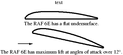
This is an example explaining \scaleput. The image appear in LaTeX companion, first edition, page 291-292, but the numbers are taken from the documentation of the curves package.
\newcommand{\RAFsixE}{
  \scaleput(1.25,1.25){\arc(0,-1.25){-135}}
  \scaleput(0,0){\curve(0.366,2.133, 1.25,3.19, 2.5,4.42,
    5.0,6.10, 7.5,7.24, 10,8.09, 15,9.28, 20,9.90, 30,10.3,
    40,10.22, 50,9.80, 60,8.98, 70,7.70, 80,5.91, 90,3.79,
    95,2.58, 99.24,1.52)}
  \scaleput(99.24,0.76){\arc(0,-0.76){180}}
  \scaleput(0,0){\curve(1.25,0, 99.24,0)}
  }
\setlength{\unitlength}{.5mm}
\linethickness{0.7mm}
\begin{center}
text\\
  \begin{picture}(100,20)
    \RAFsixE
  \end{picture}
  \\The RAF 6E has a flat undersurface.
\\
  \begin{picture}(120,30)(-20,0)
  \renewcommand{\xscale}{0.9781}
  \renewcommand{\xscaley}{0.2079}
  \renewcommand{\yscale}{0.9781}
  \renewcommand{\yscalex}{-0.2079}
  \put(0,20){\RAFsixE}
  \thicklines
  \put(-20,5){\vector(1,0){20}}
  \end{picture}
\\
  The RAF 6E has maximum lift at angles of attack over 12$^\circ$.
  \end{center}
Translation
<pic-linethickness size='0.7mm'/>
<p rend='center'>text</p>
<p rend='center'>
<picture width='142.26227' height='28.45245'>
<pic-scaleput xpos='1.77827' ypos='1.77827' xscale='1.0' yscale='1.0' xscaley='0.0' yscalex='0.0'>
<pic-arc angle='-135' xpos='0' ypos='-1.77827' unit-length='1.42262'/>
</pic-scaleput>
<pic-scaleput xpos='0' ypos='0' xscale='1.0' yscale='1.0' xscaley='0.0' yscalex='0.0'>
<pic-curve unit-length='1.42262'>0.366,2.133, 1.25,3.19, 2.5,4.42,
5.0,6.10, 7.5,7.24, 10,8.09, 15,9.28, 20,9.90, 30,10.3,
40,10.22, 50,9.80, 60,8.98, 70,7.70, 80,5.91, 90,3.79,
95,2.58, 99.24,1.52</pic-curve>
</pic-scaleput>
<pic-scaleput xpos='141.18108' ypos='1.08118' xscale='1.0'
yscale='1.0' xscaley='0.0' yscalex='0.0'>
<pic-arc angle='180' xpos='0' ypos='-1.08118' unit-length='1.42262'/>
</pic-scaleput>
<pic-scaleput xpos='0' ypos='0' xscale='1.0' yscale='1.0' xscaley='0.0' yscalex='0.0'>
<pic-curve unit-length='1.42262'>1.25,0, 99.24,0</pic-curve>
</pic-scaleput>
</picture>
</p>
<p rend='center'>The RAF 6E has a flat undersurface.</p>
<p rend='center'>
<picture xpos='-28.45245' ypos='0' width='170.71472' height='42.67868'>
<pic-put xpos='0' ypos='28.45245'>
<pic-scaleput xpos='1.77827' ypos='1.77827' xscale='0.9781'
yscale='0.9781' xscaley='0.2079' yscalex='-0.2079'>
<pic-arc angle='-135' xpos='0' ypos='-1.77827' unit-length='1.42262'/>
</pic-scaleput>
<pic-scaleput xpos='0' ypos='0' xscale='0.9781' yscale='0.9781' xscaley='0.2079' yscalex='-0.2079'>
<pic-curve unit-length='1.42262'>0.366,2.133, 1.25,3.19, 2.5,4.42,
5.0,6.10, 7.5,7.24, 10,8.09, 15,9.28, 20,9.90, 30,10.3,
40,10.22, 50,9.80, 60,8.98, 70,7.70, 80,5.91, 90,3.79,
95,2.58, 99.24,1.52</pic-curve>
</pic-scaleput>
<pic-scaleput xpos='141.18108' ypos='1.08118' xscale='0.9781'
yscale='0.9781' xscaley='0.2079' yscalex='-0.2079'>
<pic-arc angle='180' xpos='0' ypos='-1.08118' unit-length='1.42262'/>
</pic-scaleput>
<pic-scaleput xpos='0' ypos='0' xscale='0.9781' yscale='0.9781' xscaley='0.2079' yscalex='-0.2079'>
<pic-curve unit-length='1.42262'>1.25,0, 99.24,0 </pic-curve>
</pic-scaleput>
</pic-put>
<pic-thicklines/>
<pic-put xpos='-28.45245' ypos='7.11311'>
<pic-vector xdir='1' ydir='0' width='28.45245'/>
</pic-put>
</picture>
</p>
<p rend='center'>The RAF 6E has maximum lift at angles of attack over 12
<formula type='inline'>
<math xmlns='http://www.w3.org/1998/Math/MathML'>
<msup><mrow/> <mo>∘</mo> </msup>
</math>
</formula>.
</p>
Last example, showing arcs and circles.
\setlength{\unitlength}{1.8mm}
\begin{picture}(40,30)
  \thicklines
  \multiput(20,5)(20,12){2} {\line(0,-1){2}\line(-5,3){20}}
  \multiput(20,5)(-20,12){2} {\line(5,3){20}}
  \put(20,3){\line(5,3){20}}
  \put(20,3){\line(-5,3){20}}
  \put(0,15){\line(0,1){2}}
  \linethickness{1pt}
  \put(20,5) {
   \renewcommand{\xscale}{1}
   \renewcommand{\xscaley}{-1}
   \renewcommand{\yscale}{0.6}
   \renewcommand{\yscalex}{0.6}
   \scaleput(10,10){\bigcircle{10}}
   \put(0,-2){%
      \scaleput(10,10){\arc(5,0){121}}
      \scaleput(10,10){\arc(5,0){-31}}}}
\end{picture}
<picture width='204.85962' height='153.64471'>
  <pic-thicklines/>
  <pic-multiput xpos='102.42981' ypos='25.60745' repeat='2' dx='102.42981' dy='61.45789'>
    <pic-line xdir='0' ydir='-1' width='10.24298'/>
    <pic-line xdir='-5' ydir='3' width='102.42981'/>
  </pic-multiput>
  <pic-multiput xpos='102.42981' ypos='25.60745' repeat='2' dx='-102.42981' dy='61.45789'>
    <pic-line xdir='5' ydir='3' width='102.42981'/>
  </pic-multiput>
  <pic-put xpos='102.42981' ypos='15.36447'>
    <pic-line xdir='5' ydir='3' width='102.42981'/>
  </pic-put>
  <pic-put xpos='102.42981' ypos='15.36447'>
    <pic-line xdir='-5' ydir='3' width='102.42981'/>
  </pic-put>
  <pic-put xpos='0' ypos='76.82236'>
    <pic-line xdir='0' ydir='1' width='10.24298'/>
  </pic-put>
  <pic-linethickness size='1pt'/>
  <pic-put xpos='102.42981' ypos='25.60745'>
    <pic-scaleput xpos='51.2149' ypos='51.2149' xscale='1' yscale='0.6' xscaley='-1' yscalex='0.6'>
      <pic-bigcircle size='10' unit-length='5.12149'></pic-bigcircle>
    </pic-scaleput>
    <pic-put xpos='0' ypos='-10.24298'>
      <pic-scaleput xpos='51.2149' ypos='51.2149' xscale='1' yscale='0.6' xscaley='-1' yscalex='0.6'>
        <pic-arc angle='121' xpos='25.60745' ypos='0' unit-length='5.12149'>
        </pic-arc>
      </pic-scaleput>
      <pic-scaleput xpos='51.2149' ypos='51.2149' xscale='1' yscale='0.6' xscaley='-1' yscalex='0.6'>
        <pic-arc angle='-31' xpos='25.60745' ypos='0' unit-length='5.12149'>
        </pic-arc>
      </pic-scaleput>
    </pic-put>
  </pic-put>
</picture>
The \arccos command is valid only in math mode. Its translation is a math operator of the same name: <mo form='prefix'>arccos</mo>. For an example see the \log command.
The \arcsin command is valid only in math mode. Its translation is a math operator of the same name: <mo form='prefix'>arcsin</mo>. For an example see the \log command.
The \arctan command is valid only in math mode. Its translation is a math operator of the same name: <mo form='prefix'>arctan</mo>. For an example see the \log command.
The \arg command is valid only in math mode. Its translation is a math operator of the same name: <mo form='prefix'>arg</mo>. For an example see the \log command.
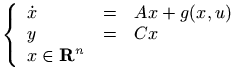
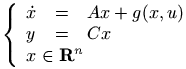
The array environment can be used only in math mode. Its first argument is a list of column specifications, where each specification is a letter, one of r, l, rc (for right justified, left justified, centered). It is followed by rows (separated by \\) and each row is a list of cells (separated by &). The eqnarray environment is implemented like an array, with rcl as specifications. In the example that follows, the outer array has only one row, and one column. The syntax of array is the same as that of tabular, but you cannot use \hline for horizontal rules, and neither | specifications for vertical rules. You may use \multicolumn.
\def\R{\mathbf{R}}
\begin{eqnarray*}
\left\{\begin{array}{lcl}
\dot{x} & = & Ax+g(x,u)\\
 y & = & Cx \\
 \multicolumn{3}{l}{x\in \R^n}
\end{array}
    \right.
\end{eqnarray*}
Translation
<formula type='display'>
<math xmlns='http://www.w3.org/1998/Math/MathML'>
<mtable>
<mtr>
<mtd columnalign='right'>
<mfenced open='{' close='.'>
<mtable>
<mtr>
<mtd columnalign='left'>
<mover accent='true'><mi>x</mi> <mo>˙</mo></mover>
</mtd>
<mtd><mo>=</mo></mtd>
<mtd columnalign='left'>
<mrow><mi>A</mi><mi>x</mi><mo>+</mo><mi>g</mi><mo>(</mo><mi>x</mi>
<mo>,</mo><mi>u</mi><mo>)</mo></mrow>
</mtd>
</mtr>
<mtr>
<mtd columnalign='left'><mi>y</mi></mtd>
<mtd><mo>=</mo></mtd>
<mtd columnalign='left'><mrow><mi>C</mi><mi>x</mi></mrow></mtd>
</mtr>
<mtr>
<mtd columnalign='left' columnspan='3'>
<mrow><mi>x</mi><mo>∈</mo><msup><mi mathvariant='bold'>R</mi>
<mi>n</mi> </msup></mrow>
</mtd>
</mtr>
</mtable>
</mfenced>
</mtd>
</mtr>
</mtable>
</math>
</formula>
We give here two versions, the old one and the new one;
in January 2005, we modified the xmt file, the result is much better.
 (see also here).
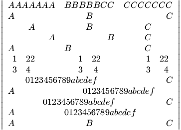
We give here another example. It shows that you can put tables into tables.
\def\MAT#1{\begin{array}{c#1}1&22\\3&4\end{array}}

\[\left|
\begin{array}{lcr}
AAAAAAA&BBBBBCC&CCCCCCC\\
A&B&C\\
\multicolumn{1}{c}{A}&\multicolumn{1}{c}{B}&\multicolumn{1}{c}{C}\\
\multicolumn{1}{r}{A}&\multicolumn{1}{r}{B}&\multicolumn{r}{c}{C}\\
\multicolumn{1}{l}{A}&\multicolumn{1}{l}{B}&\multicolumn{l}{c}{C}\\
\MAT l&\MAT c&\MAT r\\
\multicolumn{2}{c}{0123456789abcdef}&C\\
A&\multicolumn{2}{c}{0123456789abcdef}\\
\multicolumn{2}{r}{0123456789abcdef}&C\\
A&\multicolumn{2}{l}{0123456789abcdef}\\
A&B&C\\
\end{array}
\right|\]
This is half the width of the default horizontal space between columns in an array environment. It is defined in the LaTeX book class to be 5pt, so that the horizontal space is one em in a 10pt document normal size, and much smaller (in em units) for a 12pt huge size.
What Tralics should do is to add an attribute pair columnspacing='xx' to each <mtable>. The default value is 0.8em (this depends on the font size....)
Width of a vertical rule in array or tabular; not yet used by Tralics.
This command controls the spacing between rows in a table or an array. The algorithm is the following: there is an object, \strutbox, containing an invisible rule, whose height is 70% of \baselineskip and whose depth is 30% of \baselineskip (this object depends on the current font). (if \baselineskip is 12pt, this gives 8.4pt, PlainTeX defines that height to be 8.5pt).
There is another object (array-strut) constructed at the start of the array, with the same dimensions, multiplied by \arraystretch. A copy of this object is added to the start of every row. This implies that the baselines of two columns are separated by 12pt (for a ten point font, \arraystretch=1) or by 13.2pt (if \arraystretch=1.1). An expression of the the form A_1^2 has height 8.14, depth 2.48 (total 10.622) so that the vertical space between two such rows is 1.4pt by default (TeX puts a kern of value 1.6pt between the subscript and the superscript).
In MathML there is an attribute rowspacing that indicates the space between rows. The default value is 1ex (this is 4.31 pt in cmr10). This does not match the LaTeX definition.
In short: Tralics sets \arratstretch to 1, and ignores what the user does with the command.
The \Arrowvert command is an alias for \Vert.
The \arrowvert command is an alias for \vert.
The \ast command is valid only in math mode. It generates
a binary operator (looks like a *):
<mo>*</mo> (Unicode U+2A, *)
that renders like
 .
See description of the
\pm command.
.
See description of the
\pm command.
The \asymp command is valid only in math mode.
It generates a relation symbol that looks like the superposition of
\smile and \frown:
<mo>≈</mo> (Unicode U+224D, ≍)
that renders like
 .
See description of the \le command.
.
See description of the \le command.
The \AtBeginDocument command takes one argument, that is a list of tokens, which is added to the end of the document-hook token list. This list is inserted into the document when \begin{document} is executed. See description of the document environment.
This example shows the use of \AtBeginDocument and \AtEndDocument including a call to itself. In the example, the bibliography is put at the end, after the tokens inserted by \AtEndDocument. In the current version, the position of the bibliography is defined by the position of the commands \insertbibliohere or \bibliography.
\AtBeginDocument{DOC}\AtBeginDocument{S\AtBeginDocument{TART}}
\AtEndDocument{\AtEndDocument{AT\_}}
\AtEndDocument{DOC}\AtEndDocument{\_END}
The resulting XML file looks like
<?xml version='1.0' encoding='iso-8859-1'?>
<!DOCTYPE ramain SYSTEM 'raweb.dtd'>
<!-- translated from latex by tralics 2.0-->
<ramain CALC='true' creator='Tralics version2.0'>
<p>DOCSTART</p>
...
...
<p>AT_DOC_END</p></div3></div2></div1></div0>
<biblio>
...
</biblio></ramain>
The \AtEndDocument command takes one argument, that is a list of tokens, which is added to the end of the document-hook token list. The effect of the \end{document} command is to insert these tokens into the main token list. At the same moment, \AtEndDocument is made equivalent to \@firstofone (meaning: execute now). See \AtBeginDocument.
The two commands behave the same: they read an argument, and push it to the current class/package hook. This hook will be inserted when the end-of-file (corresponding to the class or package) is reached. When the command is used out of context, the hook is never inserted.
The \atop command is a TeX primitive that should not be used. Instead of `aa \atop bb' you should use `\genfrac{}{}{0pt}{}{aa}{bb}'. See \genfrac and \over.
The \atopwithdelims command is a TeX primitive that should not be used. Instead of `aa \atopwithdelims()bb' you should use `\genfrac(){0pt}{}{aa}{bb}'. See \genfrac and \over. Plain TeX defines \def\choose{\atopwithdelims()}, and you can say a\choose b. In Tralics, you would use \binom ab.