La page de J-P. Merlet

J-P. Merlet home page

La page Présentation de HEPHAISTOS

HEPHAISTOS home page

La page "Présentation" de l'INRIA

INRIA home page

Subsections

• Introduction
• The Continuation procedure
  • Optional arguments
  • Example
  
  
• Continuation with initially known starting points
• Specific parameters for the continuation procedures
• Drawing procedure

Continuation for one-dimensional system

Introduction

The purpose of continuation here is to consider a system with one parameter and $n$ unknowns and to determine what are the possible values of the unknowns when the parameters lie in a given range [a,b]. The values of the unknowns will be calculated for values of the parameter separated by a constant value, starting at one extremity of the range for the parameter.

The principle is to solve the system for the initial value a or b of the parameter range and then to obtain the solution for other values of the parameter using a certified Newton scheme (hence it is necessary that the equations of the system are at least $C^1$).

As soon as the initial starting point of the branches have been obtained the continuation procedure is usually very fast. The continuation will stop if the jacobian become singular. The algorithm will then increase the parameters value until we can start again a certified procedure.

The Continuation procedure

The full continuation procedure described in the ALIAS-C++ manual is available in Maple. It enable one to obtain initial points on the different branches of a one dimensional system and then to follow these branches. These points are written in files. The syntax of this procedure is:

 
Continuation([equation set],[variable set],[parameter name],
  [list of ranges for the variable],[range for the parameter],
  dz,epsilon,epsiloni,Sens,file base name);

where dz is the parameter increment for the storage (a point will be stored each time the parameter change value by dz), epsilon has a small value, epsiloni defines the accuracy with which the starting points of the branches are determined (if we change the parameter value of the starting point by epsiloni, then the system has no solution) and Sens is 1 if we compute the branches by increasing values of the parameter (-1 for decreasing values). Note that determining the initial starting points of the branches with an accuracy on the parameter epsiloni smaller than epsilon may a costly process: this will be done only if the flag `ALIAS/allow_backtrack` is set to 1 (its default value is 0). Note also that according to the value of Sens you may not obtain the same number of branches: Sens should be chosen so that at the initial value of the parameter (the first one for which the system has solutions) the number of solutions is maximal. A major change with respect to version 1.2 is that a backtrack mechanism is used to avoid such problem: if at some point the procedure has followed $n$ branches until a problem for Newton iteration has been detected and if the number of solutions for the next value of the parameter is $m$ with $m>n$, then the procedure will store the value of the $m$ solution and, after having completed the computation for the current Sens, will start again a continuation from this point and will follow the $m$ branch using the opposite value of Sens. Note however that only a maximum of 10 such points are stored and hence some branches may still be missing for complex expression. Note also that among the $m$ branches we will have $n$ branches that will be identical to the one that have been computed in the process before the backtrack.

The points on the branches are written in files whose names start with the file base name and is followed by the branch number. Hence if Branch is file base name and the algorithm has found two branches, then the points are written in the files Branch1, Branch2. In these files is written on each line the values of the variables in the order given by variable set followed by the value of the parameter.

By default we use only Kantorovitch theorem to follow the branches but you may also both this test and Moore test: this is done by setting the flag `ALIAS/kraw` to 1.

For this procedure the Newton scheme will be used and will run for a limited number of iteration defined by `ALIAS/newton_iteration` (default value: 100).

Note that the Draw procedure (section 7.5) allows to directly obtain a Maple plot of the branches as soon as there is only one or two unknowns.

Optional arguments

Note that optionally you may add two arguments at the end of the list of arguments. These arguments are the name of a C++ program and the name of the procedure that is defined within this program. This procedure must update the range of the unknowns according to the value of the parameter.

Assume for example that you are considering the equation:

$$(x-1)^2+(y-1)^2=l_{25}$$

where $l_{25}$ is the parameter of the system and $x,y$ the unknowns. Clearly $x$ and $y$ cannot exceed $l_{25}+1$ and cannot be lower than $-l_{25}+1$.

The syntax of this simplification procedure is:

 
int Simp(double param, INTERVAL_VECTOR v_IS)

where param is the current parameter value and v_IS the current ranges for the parameters. Unfortunately this simplification procedure cannot be produced directly by the ALIAS-Maple procedure described in chapter 4 as the argument of the simplification procedure are different.

Example

Let consider the curve described by the system:

$$\begin{eqnarray*} &&x^2-(y-1)^2+z^2-1=0\\ &&x^2-y^3=0 \end{eqnarray*}$$

where $z$ may be chosen as the parameter. To obtain in the files B1, B2, B3, B4 points of the 4 branches of this curve you will write:

 
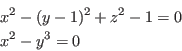
with(ALIAS):
Continuation([x^2+(y-1)^2+z^2-1,x^2-y^3],[x,y],[z],
             [[-100,100],[-100,100]],[[-2,2]],0.05,1e-6,1.e-4,1,"B");

Continuation with initially known starting points

If the starting point of branches is known it is possible to follow the branches without initially solving the system by using the procedure

 
StartContinuation(Func,Vars,Par,Init,RPar,DPar,MinD,MinI,Sens,Base,P)

where

• Func: the list of equations
• Vars: a list with the name of variables
• Par: name of the variable that will be used a parameter
• Init: a list of intervals ranges for the unknowns
• RPar: a list which define the minimal and maximal value of Par
• DPar a point is added to the plot each time the current value of Par is at DPar from the previous one
• MinD a parameter that is used to determine singular points. Its value should be small
• MinI: the accuracy on the parameter with which the initial starting point of the branch is determined: if the parameter is z and the curve start at z0, then if Sens=1 the system has no solution for z=z0-MinI
• Sens 1 is the curve is drawn from Min(Par) to Max(Par) or -1 if drawn from Max(Par) to Min(Par).
• Base a string that indicate the base-name for the files that will be created
• P: a list of starting points for the branches. For two unknowns this list has the form [[[a1,a1],[a2,a2]],...]. These points must be a solution of the system in the Kantorovitch sense and be obtained using of the solving procedure using the Hessian

A mechanism allows the user to stop the determination of a branch. For that purpose the user has to write a C++ program such as

 
 int End_Cont(MATRIX &BRANCH,int nb,int Sens, double z, INTERVAL &LIMITS)

This procedure receives the current value of the parameter (z), possible limits that have been defined for this parameters (LIMITS) and the direction (Sens) in which the value of the parameter is changed. The values of the other variables are stored in BRANCH, while their value for the current z is BRANCH(nb,...). If this procedure returns -1, then the branch will be no more followed, otherwise the procedure must return 0.

The user may indicate that such procedure is available by setting the variable `ALIAS/user_stop_continuation` to a string which indicates the name of the C++ procedure, being understood that the file that includes the code is `ALIAS/user_stop_continuation`.C

A specific procedure exists for distance equations:

 
StartContinuationDistance(Func,Vars,Par,Init,RPar,DPar,MinD,MinI,Sens,Base,P)

Specific parameters for the continuation procedures

Parameter name	Meaning	C++ equivalent
`ALIAS/allow_backtrack`	allows for backtracking the
	parameter value	ALIAS_Allow_Backtrack
`ALIAS/kraw`	allows to use the Krawczyk test	ALIAS_Use_Kraw_Continuation

Drawing procedure

For one dimensional system with 1 or 2 variables it is possible to obtain a plot of the curve. The syntax of this procedure is:

 
Draw([equation set],[variable set],[parameter name],
  [list of ranges for the variable],[range for the parameter],
  parameter increment for the storage,epsilon,epsiloni,Sens);

where the arguments are the same than the previous procedure. It returns a PLOT structure for system with one variable and a PLOT3D structure for systems with two variables. Hence to draw the previous curve you may write:

 
with(ALIAS):
with(plots):
Draw([x^2+(y-1)^2+z^2-1,x^2-y^3],[x,y],[z],[[-100,100],[-100,100]],[[-2,2]],
	0.05,1e-6,1);

Note that optionally you may add two arguments at the end of the list of arguments. These arguments are the name of a C++ program and the name of the procedure that is defined within this program. This procedure must update the range of the unknowns according to the value of the parameter.

Note that the points used for drawing the plot are stored in the file /tmp/Branch1 for the first branch, /tmp/Branch2 for the second branch and so on.

For problems involving more than 2 variables you may obtain partial plots by using the DrawND procedure, see section 9.10.

J-P. Merlet home page

La page Présentation de HEPHAISTOS

HEPHAISTOS home page

La page "Présentation" de l'INRIA

INRIA home page