The following Maple mathematical operators are recognized in an expression:
Note that the value of signum(x)=|x|/x where x is an interval
whose absolute value is lower than
`ALIAS/value_sign_signum` is set to the Maple variable
_Envsignum0. This allows one to specify the value of signum(0).
Many of the algorithm existing in the ALIAS-C++ library can be used directly from Maple. Their efficiency may be improved by using the simplification procedures described in the previous chapter.
All these procedures use the same mechanism:
All these procedures allow for an optional last argument which is the name of a simplification procedure (see chapter 4).
There are numerous parameters that allows to change the behavior of the solving procedures: they are described in the section 3.5.
int Select_Best_Direction_Interval_User(int DimVar,int DimEq,
INTERVAL_VECTOR (* TheIntervalFunction)(int,int,INTERVAL_VECTOR &),
INTERVAL_VECTOR &Input)
where DimVar is the size of the unknown vector, DimEq the number of equations, TheIntervalFunction the evaluation function of your problem (by default F)and Input the current box. This procedure shall return the variable number that will be bisected.
The boxes created after a bisection are stored in a list for further processing. There are different ways to store the new boxes:
The storage mode is controlled through the variable `ALIAS/storage_mode: 0 is used for the direct storage mode while reverse storage will be used when `ALIAS/storage_mode is set to a number equal or larger than the number of unknowns+1. Mixed storage may also be used using the variable `ALIAS/mixed_storage that indicates how many boxes are stored in place of the current box. For more details on the storage mode see the ALIAS-C++ manual.
For a specific problem the end-user may have some knowledge of the problem that implies that he may determine that for some intervals for the variables the problem has no solution, that the intervals for some variables may be reduced or that a solution may be found. Most of the ALIAS C++ solving programs have an optional argument that allows then end-user to provide this knowledge as a procedure, that will be called a simplification procedure.
Usually this procedure will take as input a set of intervals for the variables and will return an integer which is typically:
As these simplification procedures are very important for solving efficiently most problems we will devote the specific chapter 4 for those used in system solving. More specific simplification procedures will be presented together with the solving algorithms.
You may solve a system of equations and inequalities by calling the ALIAS-Maple procedures:
GeneralSolve GradientSolve HessianSolveMost of the solving procedures may deal with inequalities constraints but in the list of functions you must first define the equations and then the inequalities. For using these solvers it is needed to create C++ programs that interval evaluate the equations and their derivatives in the appropriate format. By default these procedures will use Make[FJH] to create these programs but they offer the possibility of using user's pre-defined C++ programs.
The name of the executable created by ALIAS-Maple is _GS_ but this may be changed by assigning another string to the variable `ALIAS/name_executable` or by setting the string `ALIAS/ID`.
The calculation done by these procedures may be stopped although the calculation has not been completed by setting the variable `ALIAS/time_out` to a floating point that indicates the maximum computation time in minutes. In that case the procedure will return a time out signal together with the solutions that have been obtained up to now. For example for a problem with 2 variables the message will be:
[[TIME_OUT],[[1.,1.],[2.,2.]],[[2.5,2.5],[3.,3.]]]which indicates that 2 solutions have been found before the time-out occurs.
This is the most basic procedure for solving systems. It uses only the the interval evaluation of the expressions and can deal with equations involving intervals as coefficients, while the other solving procedure cannot be used in that case.
This procedure will return as solution a set of boxes: a box is defined as a set of intervals, one for each unknowns. Such box will be obtained as soon as either the width of all the intervals is lower than `ALIAS/epsilon` or the width of the interval evaluation of the expressions for the box is lower than `ALIAS/fepsilon`. To avoid returning a large number of solutions it is assumed that all the solutions of the system are at a distance at least larger than `ALIAS/dist`.
Hence the results provided by this procedure exhibit the following features:
with(ALIAS):
u:=GeneralSolve([x^2+y^2-1,x+y],[x,y],[[-2,2],[-2,1]]);
will provide in u an approximation of the 2 solutions of the system.
The efficiency of the calculation may be improved by using a simplification procedure, see chapter 4. Hence the following code will be faster:
with(ALIAS):
HullConsistency([x^2+y^2-1,x+y],[x,y],"Simp"):
u:=GeneralSolve([x^2+y^2-1,x+y],[x,y],[[-2,2],[-2,1]],"Simp");
Note that by default when an evaluation of all the equations is needed in the C++ program, the program will proceed by successive calls to the procedure created by MakeF. This behavior may be changed by setting `ALIAS/equation_alone` to 0: in that case all equations will be evaluated by a single call to the C++ evaluation procedure. This may be important in term of computation time if the evaluation of simplification terms is performed before doing the evaluation (e.g. if the procedure ALIAS_FSIMPLIFY has been defined, see the MakeF section 2.1.1).
Note that there is a specific bisection mode that can be used for this solving algorithm. The table `ALIAS/table_ordered_bisection`, with as many lines as equations, will contain variable number in a row such as for the first row [1,3,4]. This will indicate that only variables 1, 3, 4 will first be bisected until the first equation is satisfied. Then we will move to the second equation and the second row of the table. This bisection method is validated as soon as the flag `ALIAS/ordered_bisection` is set to 1.
The syntax of these procedures is the same as GeneralSolve but there are two main differences between these procedures and GeneralSolve:
When ALIAS has returned a point M as solution it is always possible to retrieve the boxes in which it was found that there was a unique solution whose approximation is M: all interval solutions are available via the list `ALIAS/Solutions`.
In spite of the additional computation time involved by the use of the derivatives, these procedures are in general faster than GeneralSolve. Indeed the algorithms that are used in these procedures may allow to determine relatively large box in which an unique solution will be found, thereby avoiding a large number of bisection. As this knowledge is used to manage the list of boxes it may have a drastic effect on the computation time of the algorithm.
Note that it is possible to avoid using the Hessian (which may be computer intensive) for the evaluation of the expressions by setting the variable `ALIAS/no_hessian` to 1. The flag `ALIAS/rand` may be used to switch of bisection mode from time to time (it fixes the value of the ALIAS-C++ ALIAS_RANDG variable). The variables `ALIAS/size_tranche_bisection` and `ALIAS/tranche_bisection` may be used for the bisection mode 8 of GradientSolve (see the ALIAS-C++ manual).
For systems with ![]() equations and
equations and ![]() unknowns with
unknowns with ![]() the
algorithm computes the exact solutions of the first
the
algorithm computes the exact solutions of the first ![]() equations. Then
if the interval evaluation of all the
equations. Then
if the interval evaluation of all the ![]() remaining equations has an
absolute value lower than `ALIAS/fepsilon` the solution is
supposed to be valid. For systems with
remaining equations has an
absolute value lower than `ALIAS/fepsilon` the solution is
supposed to be valid. For systems with ![]() see
section 3.4.
see
section 3.4.
ALIAS-Maple provides solving procedures for systems having specific structures.
This procedure allows to solve systems that have algebraic terms in at least at two equations. Each equation is transformed as the sum of a linear part and a non linear part. The linear part is substituted into a new variable that is submitted to a linear constraints. Then the simplex method is used to improve the range for the unknowns. The difference between the SolveSimplex and SolveSimplexGradient procedure is that in the second case the derivatives of the non linear parts of the equations are used to improve their interval evaluation and hence the linear constraints used by the simplex.
The following variables plays a role in these procedures:
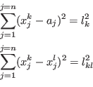
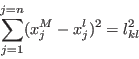
The SolveDistance procedure allows to solve systems of distance
equations. A distance equation describes that the distance between
m points in a n-dimensional space is given. The unknowns are the
n coordinates
![]() of the points. Hence a distance
equation may be written
as:
of the points. Hence a distance
equation may be written
as:

SolveDistance(Func,Vars,Init)The initial search domain for SolveDistance may be determined using the Bound_Distance procedure.
Note that there is no need to use the HullConsistency simplification procedure when using SolveDistance as it is already embedded in the C++ method. The consistency method in the algorithm updates the value of the variables and starts again the update if the change in at least one interval exceed the threshold `ALIAS/seuil2B` (which has the default value 0.1).
As the SolveDistance algorithm uses systematically a Newton
scheme with as estimate of the solution the center of the box, it may
be interesting to switch the current box with the largest one in the
list of boxes to process in order to find new solutions to the system
very quickly. Indeed if the Newton scheme appears to converge toward
an approximate solution ![]() we will
use a special version of the Kantorovitch test to determine a box
we will
use a special version of the Kantorovitch test to determine a box
![]() centered at
centered at ![]() that contains only one solution. This box will be
further enlarged by using a specific version
of the Neumaier
test (this is called an inflation of the box). Then we will
determine if
that contains only one solution. This box will be
further enlarged by using a specific version
of the Neumaier
test (this is called an inflation of the box). Then we will
determine if ![]() has an intersection with each box
in the list of boxes to process and if this is the case we will modify
the list of boxes so that it has only boxes that are the complementary
of
has an intersection with each box
in the list of boxes to process and if this is the case we will modify
the list of boxes so that it has only boxes that are the complementary
of ![]() : this process will speed up the algorithm.
: this process will speed up the algorithm.
Switching the current box with the largest one is done by setting the flag `ALIAS/permute` to the number of bisection after which the boxes will be permuted. The default value for this flag is 1000 and if it is set to 0 no permutation will be done.
Note that if you have a system of distance equations with one
parameter, you may fix the value of this parameter to a given value ![]() and then follow the solutions when the parameter changes in the range
[
and then follow the solutions when the parameter changes in the range
[![]() ] by using a specific continuation procedure (see
section 7.3)
] by using a specific continuation procedure (see
section 7.3)
Let consider the family of linear systems defined by the matrix equality
The enclosure can be computed using the LinearBound procedure whose syntax is
LinearBound(A,B,Derivative,Vars,Init)where:
with(ALIAS):
with(linalg):

A:=array([[x,y],[x,x]]):
B:=array([x,y]):
VAR:=[x,y]:
LinearBound(A,B,0,[x,y],[[3,4],[1,2]]);
LinearBound(A,B,1,[x,y],[[3,4],[1,2]]);
which returns the enclosure [[.76923076923077, 10], [-13, -.076923076923077]] if Derivative is set to 0 and [[.91666666666667, 2.6666666666667], [-2, -.66666666666667]] if Derivative is set to 1 (note that these values are computer dependent), the exact answer being [[1.25,1.66666],[-1]].
We consider a matrix whose coefficients are functions of a set of variables. The procedure RegularMatrix allows one to determine if the set of matrices includes only regular matrices. Its syntax is
RegularMatrix(mat,vars,init,cond,typedet)where
Note that the procedure generates the C++ code for calculating the elements of the matrix by using the procedure MakeF. If these elements includes several times the same complex expressions it is advised to use the mechanism described in MakeF (section 2.1.1) to interval evaluate these expressions only once.
Note also that the used bisection method is to bisect the unknown range having the largest width. Scaling the unknown is therefore important
Note a special case that may occur if the matrix may include interval coefficients apart of the parameters or if the matrix is badly numerically conditioned. In that case it may happen that for a specific value of the parameters the sign of the determinant of the matrix cannot be ascertained (such point will be called unsafe). Hence at this point we cannot state the regularity of the matrix. But it may happen that at 2 other points the determinants will have opposite sign indicating the presence of a singularity. So the following cases may occur:
The procedure may behave in 2 different ways:
The procedure behavior is controlled through the flag `ALIAS/unsafe_det`. If this flag is set to 1 behavior 1 will be used while behavior 2 is obtained by setting the flag to 0. The default value of this flag is 0. For behavior 1 the return code of the procedure is -3 if an unsafe point is found.
The procedure reorders the boxes every `ALIAS/rand` iteration (default value=0 i.e. at each iteration). The ordering may be controlled through the `ALIAS/order` variable. Assume that the interval evaluation for a box is [a,b]. At some point the procedure will have find a box with a constant sign s for the determinant:
The conditioning may play an important role especially as the conditioned matrix is calculated symbolically. Assume for example that the first row of A is [x x] and that AK is used. If the first column of K is [a1 a2], then the first element of the conditioned matrix is a1x+a2x, that the procedure will arrange as x(a1+a2), thereby leading to an optimal form in term of interval evaluation, which is better than the numerical conditioning.
The procedure accepts an optional sixth argument which is a string such as SIMP that defines a matrix simplification procedure. The syntax of such procedure is
SIMP(int dimA,INTERVAL_MATRIX & A)where dimA is the dimension of matrix A. This procedure shall return -1 if all the matrices in the set A are regular, 0 otherwise. The C++ program corresponding to this procedure is written in the file SIMP.C. Such program may be obtained for example by using the RohnConsistency or SpectralRadiusConsistency procedures.
A parallel version of this procedure is ParallelRegularMatrix.
RohnConsistency(name)where name indicates the name of the procedure, that will be written in the file name.C. This simplification procedure uses Rohn regularity test that is based on the calculation of
Note that if the flag Use_Simp_Cond is set to 0 this test will not be used if the C++ flag Simp_In_Cond is not equal to 0. For example in RegularMatrix this is the case if the matrix received by Rohn is a conditioned matrix.
A remembering mechanism may allow to reduce the computation time by storing information on already processed matrix in the Rohn test. For using this mechanism you must set `ALIAS/rohn_remember` to the number of matrix that will be stored and `ALIAS/rohn_size_matrix` to the dimension of the matrix.
SpectralRadiusConsistency(name,eps,iter)where name indicates the name of the procedure, that will be written in the file name.C. The floating point eps is used to compute a safe upper bound of the spectral radius: usually a value of
Note that if the flag Use_Simp_Cond is set to 0 this test will not be used if the C++ flag Simp_In_Cond is not equal to 0. For example in RegularMatrix this is the case if the matrix received by the procedure is a conditioned matrix.
This procedure should be used in conjunction with RegularMatrix. It should be used only if the matrix includes rows or columns in which a variable appears with degree 1 in at least 2 elements of a row or a column. Its syntax is:
 LinearMatrixConsistency(A,VAR,vars,row,context,rohn,
                        Func,FuncKA,FuncAK,name)
The parameters are:
x xy x+ythis row may be considered as linear in x in which case we have 3 linear elements in the row. If the row is considered as linear in y we have 2 linear elements in the row. Note that the linearity is checked according to the order provided in Vars.
This procedure may be used for the matrix A, the conditioned matrix KA or the conditioned matrix AK. Context is used to indicate the choice according to the following code:
For example we may use
LinearMatrixConsistency(A,[x,y],[x],1,5,"F","AKA","","Simp"):In this example we will consider the row of matrix A and its elements that are linear in x. The procedure will be used for both the matrix A and the conditioned matrix KA (hence this procedure should be used with the parameter cond of RegularMAtrix set to 1 or 3. Note that we assume here that the conditioning matrix is
Any ALIAS maple procedure involved in the calculation on eigenvalues of a matrix A may use the Gerschgorin circles methods that states that all the eigenvalues of a matrix are enclosed in the union of a set of circles (in the complex plane) whose center and radii are calculated as functions of the coefficients of the matrix.
The purpose of the GerschgorinConsistency procedure is to generate the C++ code for a simplification procedure that may be used by the ALIAS-Maple procedures doing calculation on the eigenvalues of a square matrix. The syntax is:
GerschgorinConsistency(Func,Vars,Gradient,n,procname)where:
To check only if the eigenvalues lie in the interval provided by the C++ procedure without modifying this interval use a negative n
Although the solving procedures of ALIAS are mostly devoted to be used for 0 dimensional system (i.e. systems having a finite number of solutions) most of them can still be used for non 0-dimensional system. Specific procedures for systems of dimension 1 are described in chapter 7. For larger dimension systems the solving procedures of ALIAS-Maple will provide an approximation of the result as a set of input intervals that are written in a file. To deal with non-0 dimensional system it is necessary to set the flag `ALIAS/ND` to 1 and to set the name of the file in the variable `ALIAS/ND_file` (its default value is .resultND.
The total volume of the boxes written in the file may be obtained through the variable `ALIAS/VolumeIn`. During the process we call neglected boxes the boxes that cannot be eliminated as not containing solutions of the problem but can neither be discarded as part of the boxes may contain a solution. A box will be neglected if its width is lower than `ALIAS/epsilon`. The total volume of the neglected boxes may be obtained through the variable `ALIAS/VolumeNeglected`.
The result (or cross-sections of it if the problem has more than 3 variables) may be visualized using the DrawND procedure described in section 9.10.
The behavior of the solving algorithms may be adjusted using various parameters that are presented in the on-line help (see ALIAS[Parameter]): basically all the parameters that may be adjusted in the C++ library may be also adjusted via Maple.
| Parameter name | Meaning | C++ equivalent |
| `ALIAS/debug` | flag for debug purpose | Debug_Level_Solve_General_Interval |
| `ALIAS/dist` | minimal distance between 2 distinct | |
| solutions (for GeneralSolve) | ||
| `ALIAS/epsilon` | maximal width of a solution box | |
| `ALIAS/fepsilon` | maximal width of the expressions | |
| evaluation for a solution box | ||
| `ALIAS/lib` | string that indicates the | |
| location of the ALIAS C++ library | ||
| `ALIAS/maxbox` | maximal number of stored boxes | |
| `ALIAS/maxsol` | maximal number of solutions | |
| `ALIAS/rand` | allow to switch between | |
| bisection modes | ALIAS_RANDG | |
| `ALIAS/rand` | exchange largest box with | |
| current every xx iter. | ALIAS_RANDG | |
| `ALIAS/mixed_bisection` | bisection mode, see section 3.1.3 | ALIAS_Mixed_Bisection |
| `ALIAS/mixed_storage` | allows to switch between | Switch_Reverse_Storage |
| direct and reverse storage | ||
| `ALIAS/optimized` | flag to indicate if the C++ | |
| files are compiled with -O | ||
| `ALIAS/order` | ordering for the storage of | |
| the boxes, | ||
| see the ALIAS-C++ manual | ||
| `ALIAS/profil` | string that indicates the | |
| location of the BIAS/Profil library | ||
| `ALIAS/single_bisection` | bisection mode, see section 3.1.3 | Single_Bisection |
| `ALIAS/storage_mode` | bisection mode, see section 3.1.4 | Reverse_Storage |
| `ALIAS/name_executable` | name of the executable | |
| `ALIAS/allows_n_new_boxes` | maximum number of boxes | |
| that can be created | ||
| when intersecting a box | ||
| and a unicity box | ALIAS_Allows_N_New_Boxes | |
| `ALIAS/type_n_new_boxes` | if the maximum number of boxes | |
| that is created | ||
| when intersecting a box | ||
| and a unicity box | ||
| is lower than the maximum | ||
| determine the rule to create | ||
| the new boxes (see ALIAS-C++) | ||
| `ALIAS/tranche_bisection` | for bisection mode 8 | ALIAS_Tranche_Bisection |
| `ALIAS/size_tranche_bisection` | for bisection mode 8 | ALIAS_Size_Tranche_Bisection |
The variable `ALIAS/stop_first_sol` allows to exit from a solving procedure without completing the full calculation. The following behavior will be obtained according to the value of this flag:
For the expression involving the determinant of a matrix we have some specific variables:
| Parameter name | Meaning | C++ equivalent |
| `ALIAS/det22` | see section 2.1.3 | |
| `ALIAS/minor22` | see section 2.1.3 | |
| `ALIAS/row22` | see section 2.1.3 |
You may also directly obtain a full program for one of the three main solving procedures of ALIAS by setting the variable `ALIAS/runit` to 0.
You may then compile the created program using the makefile _makefile. These procedures may be used with inequality constraints. Alternatively you may run Maple with a solving program embedded in the Maple code and stop the session when the compilation starts. According to the algorithm you are using the name of the main program will start with _G and has the extension .C (alternatively you may define the name of the main program using the variable `ALIAS/name_executable`) Alternatively you may define a string in `ALIAS/ID` and all files that will be created during the solving process will have this string appended to their name.
jean-pierre merlet