INRIA home page
Subsections
A parametric polynomial is a polynomial whose coefficients are
functions of a set of parameters (in other words it is a set of
polynomials). A typical parametric polynomial is obtained when
calculating the characteristic polynomial of a parametric matrix.
In this chapter we propose some algorithms to deal with the real roots
of a parametric polynomial and, in some cases, with the real part of
these roots. If the considered polynomial is the characteristic
polynomial of a matrix we may make use of the components of the
matrix.
Some of these algorithms use a primary and secondary algorithms. The
secondary algorithm uses also a list of boxes which is stored in the
interval matrix BoxUP.
Minimal and maximal real roots of a parametric polynomial
The purpose here is to determine the minimal and maximal values of the
set of real roots of the the set of polynomials, when the parameters
are bounded. There may be eventually also constraints on the
parameters.
The algorithm is implemented as:
int ALIAS_Min_Max_EigenValues(int Degree,
                              int Nb_Parameter,
                              INTERVAL_VECTOR (* TheCoeff)(INTERVAL_VECTOR &),
                              int Nb_Constraints,
                              INTEGER_VECTOR &Type_Eq,
                              int (* TheMatrix)(INTERVAL_VECTOR &, INTERVAL_MATRIX &),
                              int Has_Matrix,
                              INTERVAL_VECTOR (* IntervalFunction)(int,int,INTERVAL_VECTOR &),
                              int *Has_Gradient,
                              INTERVAL_MATRIX (* Gradient)(int, int,INTERVAL_VECTOR &),
                              INTERVAL & TheDomain,
                              INTERVAL_VECTOR & TheDomain_Parameter,
                              int Type,int Nb_Points,int Use_Solve,int rand,
                              int M,
                              double Accuracy_Variable,double Accuracy,double AccuracyM,
                              INTERVAL &Lowest_Root,INTERVAL &Highest_Root,
                              INTERVAL_MATRIX &Place,int  Stop,double *Seuil,
                              int (* Solve_Poly)(double *, int *,double *),
                              int (* Simp_Proc)(INTERVAL_VECTOR &))
where the arguments are:
- Degree: degree of the polynomial
- Nb_Parameter: number of parameters appearing in the
coefficients
- TheCoeff: a procedure that take as input an interval
vector and returns the interval value of the coefficients of the
polynomial. The elements of the input interval vector are first a
range for the unknown in the polynomial, then the ranges for the Nb_Parameter parameters
- Nb_Constraints: the number of constraints expression that
constraints the parameters
- Type_Eq: type of the constraints expressions (0 for
equality, -1 for inequality of type
 0, 1 for inequality of type
 0)
0)
- TheMatrix: the polynomial may be the characteristic
polynomial of a matrix
 . This argument is a procedure that takes
as first argument the
same interval vector as TheCoeff and returns in the second
argument the interval component of . This procedure must return 1
if the components have been successfully calculated, -1 otherwise
. This argument is a procedure that takes
as first argument the
same interval vector as TheCoeff and returns in the second
argument the interval component of . This procedure must return 1
if the components have been successfully calculated, -1 otherwise
- Has_Matrix: this flag must be set to 0 except if the
polynomial is the the characteristic
polynomial of a matrix in which case it must be set to 1 (2 if the
matrix is symmetrical)
- IntervalFunction: a function which return the interval
vector evaluation of the constraints and of the polynomial, the last
component of the vector being the interval evaluation of the
polynomial. This procedure must be written in ALIAS standard form, see
note 2.3.4.3
- Has_Gradient: an array of integer that indicates if the
derivatives of the expression are available. Only the first element is
used for now with the following value:
- 0: no derivative available
- 1: only the derivatives of the constraints are
available, not the one of the polynomial
- 2: all derivatives are available
- Gradient:a procedure which returns the Jacobian matrix of
the expression for given values of the unknowns written in standard
ALIAS form (see note 2.4.2.2)
- TheDomain: range for the polynomial unknown. This range
must be large and is automatically adjusted during the calculation
- TheDomain_Parameter: the ranges for the parameters
- Type: 0 for finding only the minimum of the real root, 1
to find only the maximal root and 2 to find both
- Nb_Points: to estimate the minimal and maximal real root
the algorithm compute the root of the polynomial at some given points
for which the parameters have a fixed value. This value give the
number of points where this procedure is used, it must be at least 1.
- Use_Solve: if this parameter is 1 or 3, then for each box
we try to determine bounds for the real roots using algebraic
geometry. If it is 2 or 3 then for each box we solve numerically the
polynomial for
some specific values of the parameters to update the minimum and
maximum. If the value is 0 or 1 we will assume that a root of a
polynomial is obtained when the width of the box is lower than Accuracy_Variable and the width of the evaluation of the polynomial
is lower than Accuracy. If the confidence in the routine that
solve numerically a polynomial is low the best choice is 1 otherwise
the best choice is 3
- rand: every rand iteration the algorithm will
consider that the current box is the one in the list that has the
largest width. Such random permutation may allow to determine the
minimal and maximal real root more quickly. This number must be
neither
too low (otherwise the maximal memory available may be exceeded) nor
too large (otherwise the algorithm may focus on some part of the
search space while the optimum is located in another part). A good
compromise is 100.
- M: the maximum number of boxes which may be
stored. See the note 2.3.4.5
- accuracy_Variable: the maximal width of the range of the
polynomial unknown to be a solution, see the
note 2.3.4.6
- Accuracy: the maximal width of the polynomial evaluation for
a solution, see the
note 2.3.4.6
- AccuracyM: the accuracy with which the optimum is
determined. The absolute value of the difference between the real
optimum and the calculated one should not
exceed this value
- Lowest_Root, Highest_Root: point interval
giving the minimal and maximal
real root
- Place: the value of the parameters for which the optimum
is obtained: the first line is for the minimum and the second line for
the maximum
- Stop, Seuil: if Stop is set to 1
- when looking for a minimum only the procedure exit as
soon as a minimum lower than Seuil[0] has been found
- when looking for a maximum only the procedure exit as
soon as a maximum greater than Seuil[1] has been found
- when looking both for a minimum and a maximum the
procedure exit as a minimum lower than Seuil[0]
OR a maximum greater than Seuil[1] has been found
If Stop is set to 2 when looking both for a minimum and a maximum the
procedure exit as a minimum lower than Seuil[0]
AND a maximum greater than Seuil[1] has been found (otherwise as
the same behavior than 1)
- Solve_Poly: a procedure that compute the real roots of a
polynomial. It takes as argument the coefficients of the polynomial, a
pointer to an integer that is initially the degree of the polynomial
and the real roots are stored in the last argument. This
procedure returns the number of real roots or -1 if the computation
has failed. ALIAS provides as possible procedure ALIAS_Solve_Poly.
- Simp_Proc: a user-supplied procedure that take as input
the current box and may proceed to some reduction of
the width of the box or even determine that there is no
solution for this box, in which case it should return
-1.
The confidence in this procedure is at the same level than the
confidence in the numerical algorithm that solve a polynomial.
The return code is:
- 1: algorithm has succeeded
- 0: result is not guaranteed
- -1: algorithm has failed, not enough memory
- -2: largest root of the polynomial lower than the given lower
bound
- -3: smallest root of the polynomial larger than the given upper
bound
- -4: error in the type of the equations
- -5: error, more than one function to optimize
- -100: in the mixed bisection mode the number of variables
that will be bisected is larger than the number of unknowns
- -150: ALIAS_Delta3B or
ALIAS_Max3B have not the right dimension Nb_Parameter+1
- -200: one of the value of ALIAS_Delta3B or
ALIAS_Max3B is negative or 0
- -300: one of the value of ALIAS_SubEq3B is not 0 or 1
- -1000: Single_Bisection has an incorrect value
- -1500: Degree is lower than 0
- -2000: Nb_Parameter is lower or equal to 0
- -3000: we use the full bisection mode and the problem has
more than 10 unknowns
- -3500: Nb_Constraints is lower than 0
- -4000: Type not between 0 and 2
- -4500: Stop_First_Sol not between 0 and 2
- -5000: Use_Solve not between 0 and 4
- -6000: Place has not 2 rows or Nb_Parameter+1
columns
- -6500: the initial estimate have incompatible lower and upper
bound
The possible bisection mode are:
- 1: if the polynomial parameter has a value that is better than
the current optimum, then this variable is bisected otherwise mode 1
of section 2.4.1.3
- 2: mode 1 of section 2.4.1.3 if the gradient is not available
- 3,4: mode 1 of section 2.4.1.3
- 5: mode 5 of section 2.4.1.3
For mode 2 if the gradient is available and if the polynomial parameter
has a value that is better than
the current optimum, then this variable is bisected otherwise we use
the smear function to determine the bisected variable.
It may be of interest to determine what may be the possible values of the
parameters of a parametric polynomial such that the real roots of the
corresponding polynomial are all enclosed in a given interval. ALIAS provides two routines for that purpose.
Let consider the parameters space i.e. a  dimensional space
where each of the dimension corresponds to one of the
parameters.
A point in this space corresponds to a unique value for all the
parameters and therefore to a specific polynomial.
In the parameters space there are possibly a set
dimensional space
where each of the dimension corresponds to one of the
parameters.
A point in this space corresponds to a unique value for all the
parameters and therefore to a specific polynomial.
In the parameters space there are possibly a set  of regions such that
for any point in the region(s) the corresponding polynomial has all
its root within the given interval. The purpose of the following
procedure is to determine an approximation of . This
approximation
of regions such that
for any point in the region(s) the corresponding polynomial has all
its root within the given interval. The purpose of the following
procedure is to determine an approximation of . This
approximation  will be constituted of a set of dimensional boxes
which are guaranteed to be included in and that will be
written in a file. During the calculation the boxes whose width is
lower than a given threshold
will be constituted of a set of dimensional boxes
which are guaranteed to be included in and that will be
written in a file. During the calculation the boxes whose width is
lower than a given threshold  and for which the algorithm
has been unable to determine if they are fully enclosed in
will be neglected. A possible index for measuring the quality of the
approximation is the ratio
and for which the algorithm
has been unable to determine if they are fully enclosed in
will be neglected. A possible index for measuring the quality of the
approximation is the ratio  between the total
volume
between the total
volume  of the boxes
written into the file over the total volume
of the boxes
written into the file over the total volume  of the boxes that have
been neglected as the volume of is lower or equal to
of the boxes that have
been neglected as the volume of is lower or equal to  .
.
The procedure is:
int ALIAS_Min_Max_EigenValues_Area(int Degree,int Nb_Parameter,
          int Has_Interval,
          INTERVAL_VECTOR (* TheCoeff)(INTERVAL_VECTOR &),
          INTERVAL_VECTOR (* TheCoeffCentered)(INTERVAL_VECTOR &,double),
          int Nb_Constraints,INTEGER_VECTOR &Type_Eq,
          int (* TheMatrix)(INTERVAL_VECTOR &, INTERVAL_MATRIX &),
          int Has_Matrix,
          INTERVAL_VECTOR (* IntervalFunction)(int,int,INTERVAL_VECTOR &),
          int Has_Gradient,
          INTERVAL_MATRIX (* Gradient)(int, int,INTERVAL_VECTOR &),
          INTERVAL & TheDomain,INTERVAL_VECTOR & TheDomain_Parameter,
          int Nb_Points,int Use_Solve,int rand,int Strong,int Iteration,
          double Accuracy_Variable,double Accuracy,double AccuracyM,double AccuracyB,
          double *Volume_Result,double *Volume_Neglected,double Seuil,
          char *FileName,int Has_Input,char *File_Input,
          int (* Solve_Poly)(double *, int *,double *),int RealRoot,
          INTERVAL_VECTOR (* Evaluate_Complex)(int,int,INTERVAL_VECTOR &),
          int (* Simp_Proc)(INTERVAL_VECTOR &))
where the arguments are similar to the one of the previous procedure
except for:
- TheCoeffCentered: a procedure that returns the coefficients
in x of the polynomial P(x+a). Takes as argument the parameters vector
and a
- AccuracyB: the threshold for the maximal width
of the neglected boxes
- Volume_Result: the total volume of the boxes that have
been determined to be enclosed in the regions
- Volume_Neglected: the total volume of the boxes that have
been neglected
- Seuil: the interval [Seuil[0], Seuil[1]] defines the
allowed range for the real roots of the polynomial
- FileName: the name of the file in which will be written
the boxes that are included in the regions
- Has_Input, File_Input: the purpose of these
variables is to allow an incremental improvement of the
approximation. Indeed after a first run with a given the
quality index may be not satisfactory. It is possible to improve it by
decreasing the value of for a second run but it means that
the boxes that have been determined to be enclosed in the region
during the first run will be considered again, thereby leading to a
loss of efficiency. These arguments allow a better control. During the
first run if Has_Input has been set to 1 the neglected boxes
will be stored in the file File_Input. During the second run
(and the subsequent run if needed) Has_Input will be set to 2
and the set of boxes to be considered by the algorithm will be read
from the file File_Input. During this type of run the neglected
boxes will still be written in the file, allowing another run of the
algorithm if needed. Hence the total volume of the boxes enclosed in
the region will be the sum of the Volume_Result while the total
volume of the neglected boxes will be the obtained during the last run
of the algorithm. If Has_Input is set to 3 the neglected boxes
will not be saved in a file.
- Strong: if 1 we use a secondary algorithm to determine if
for a given box all the polynomial roots are in the range
- RealRoot: 0 if we are considering only real roots, 1 for
the real part of the roots, 2 if we consider polynomial whose roots
are all real and 3 if we consider polynomial with at least one real
root
- Evaluate_Complex(i1,i2,X: let P be the polynomial and
U=P(Seuil_First_Sol[0]+I b), V=P(Seuil_First_Sol[1]+I b). Let
 be the real part of U,
  the complex part of U,
  the real
part of V and
the real
part of V and  the complex part of V. The procedure will return
in its interval vector the value of
the complex part of V. The procedure will return
in its interval vector the value of  to
to  . X
is a Nb_Parameter+1 interval vector, the last one being
the value of b
. X
is a Nb_Parameter+1 interval vector, the last one being
the value of b
This procedure returns the number of boxes written in the result file
or a negative number if the calculation has failed.
The possible negative return code are:
- -2, -3: errors on the bounds for the roots
- -10: Iteration is lower than 10
- other values: the procedure that compute the minima and maximal
real rots in a box has failed
This second procedure allows to compute the largest square (up to a
pre-defined accuracy  ) that is enclosed in the region. This
largest box
can clearly be obtained from the result of the previous algorithm but
this weaker procedure will be faster.
) that is enclosed in the region. This
largest box
can clearly be obtained from the result of the previous algorithm but
this weaker procedure will be faster.
The principle is to have a set of boxes whose first element is a range
for the center of the box and second element is a possible value for
the length of the half-edge of the square. The main algorithm will
test if for a given box the center may be a candidate to be the center
of a square of half-edge  (where
  is the current optimum)
using some heuristics and if the answer is
positive will compute the minimal and maximal root of the polynomials
defined by this square using a secondary algorithm. If these values
are compatible with the bound
the current optimum will be updated.
is the current optimum)
using some heuristics and if the answer is
positive will compute the minimal and maximal root of the polynomials
defined by this square using a secondary algorithm. If these values
are compatible with the bound
the current optimum will be updated.
int ALIAS_Geometry_Carre(int Degree,int Nb_Parameter,
           INTERVAL_VECTOR (* TheCoeff)(INTERVAL_VECTOR &),
           int Nb_Constraints,INTEGER_VECTOR &Type_Eq,INTEGER_VECTOR &Imperatif,
           int (* TheMatrix)(INTERVAL_VECTOR &, INTERVAL_MATRIX &),
           int Has_Matrix,
           INTERVAL_VECTOR (* IntervalFunction)(int,int,INTERVAL_VECTOR &),
           int *Has_Gradient,
           INTERVAL_MATRIX (* Gradient)(int, int,INTERVAL_VECTOR &),
           INTERVAL & TheDomain,INTERVAL_VECTOR & TheDomain_Parameter,
           int Nb_Points,int Use_Solve,int rand,
           int Iteration_Geometry,int Iteration_Polynom,
           double Accuracy_Variable,double Accuracy,double Accuracy_Geometry,
           double Accuracy_Polynom,INTERVAL_VECTOR &Solution,double *Seuil,
           int (* Solve_Poly)(double *, int *,double *),
           int (* Simp_Proc)(INTERVAL_VECTOR &),
           int (* Simp_Proc_Pol)(INTERVAL_VECTOR &))
The arguments are the same than for the previous procedure except for:
- Imperatif: an array of integer. If there are constraints
that are imperative, meaning that the polynomial cannot be evaluated
if they are not satisfied (for example the constraints is that some
term is positive as in the coefficients of the polynomial this term
appears as a square root) you may set the corresponding integer to
1. If this array has dimension 0 all the constraint will supposed to
be not imperative
- Iteration_Geometry: the number of boxes that may be used
by the main algorithm
- Iteration_Polynom: the number of boxes that may be used
by the secondary algorithm
- Accuracy_Geometry: the value of
- Accuracy_Polynom: the accuracy used for the secondary
algorithm. Note that this parameter play a role not only on the
computation time but also on the bound for the root. Indeed the
algorithm will verify that in the square there is no polynomial with a
root lower than Seuil[0]+Accuracy_Polynom or larger than Seuil[1]-Accuracy_Polynom
- Solution: the point interval is the center of the largest
square while the second is the value of the half-edge
- Simp_Proc: a simplification procedure used only in the
main algorithm. The flag ALIAS_Simp_Main is set to 1 when this
procedure is called right after the bisection process.
- Simp_Proc_Polynom: a simplification procedure used only in the
secondary algorithm
This procedure will return:
- -1000: error in the Single_Bisection flag that should be
between 0 and 5
- -4: error in Type_Eq
- -3: the lowest root of all the polynomials is greater than Seuil[1]
- -2: the highest root of all the polynomials is lower than Seuil[0]
- -1: the algorithm has failed
- 0: the result is not guaranteed
- 1:the result is guaranteed
During the calculation the flag ALIAS_Has_OptimumG will be set
to 1 as soon as an optimum is found: the center of the current optimal
geometry is the mid point of the interval vector ALIAS_Vector_OptimumG while is edge is in the interval ALIAS_OptimumG.
The secondary algorithm uses the flag Single_BisectionG and
Reverse_StrorageG that play the same role than Single_Bisection and Reverse_Storage in the general solving
algorithms (see sections 2.3.1.3 and 2.3.1.2).
The condition number of a polynomial may be defined either
as the ratio lowest root over largest root or as the ratio
 over
over
 where
where  are the roots of the
polynomial. In the later case the condition number has a value between
0 and 1.
The minimal and maximal values of the condition number of a parametric
polynomial in both form may be calculated using the procedure:
are the roots of the
polynomial. In the later case the condition number has a value between
0 and 1.
The minimal and maximal values of the condition number of a parametric
polynomial in both form may be calculated using the procedure:
int ALIAS_Min_Max_CN(int Degree,
     int Nb_Parameter,INTERVAL_VECTOR (* TheCoeff)(INTERVAL_VECTOR &),
     int Nb_Constraints,INTEGER_VECTOR &Type_Eq,
     int (* TheMatrix)(INTERVAL_VECTOR &, INTERVAL_MATRIX &),
     int Has_Matrix,
     INTERVAL_VECTOR (* IntervalFunction)(int,int,INTERVAL_VECTOR &),
     int Has_Gradient,
     INTERVAL_MATRIX (* Gradient)(int, int,INTERVAL_VECTOR &),
     INTERVAL & TheDomain,INTERVAL_VECTOR & TheDomain_Parameter, int Type,
     int Nb_Points,int Absolute,
     int rand,int Iteration,
     double Accuracy_Variable,double Accuracy,double AccuracyM,
     INTERVAL &Lowest,INTERVAL &Highest,
     INTERVAL_MATRIX &Place,int  Stop, double *Seuil,
     int (* Solve_Poly)(double *, int *,double *),
     int (* Simp_Proc)(INTERVAL_VECTOR &))
where the arguments are identical than for the previous procedure
except for:
- Absolute: 0 if looking for the ratio minimal root over
maximal root, 1 if looking for the ratio in absolute value
- AccuracyM: the accuracy with which the ratio will be
computed
- Lowest, Highest: minimal and maximal value of the
condition number
This procedure allows for the calculation of the minimal and maximal
condition number of a matrix.
Various bisection methods are available through the use of the integer
Single_Bisection:
- 1: mode 1 of section 2.4.1.3
- 2: mode 6 of section 2.4.1.3 if the gradient is not available
- 3,4: mode 1 of section 2.4.1.3
- 5: mode 5 of section 2.4.1.3
A specific procedure is used when the gradient is available. If the
interval for the root includes 0 we bisect it. Otherwise we use the
smear function to decide which other variable should be bisected.
Kharitonov
polynomials are special polynomials that have constant values for their
coefficients and are associated to a parametric polynomial.
It can be shown that if all the Kharitonov polynomials have
the real parts of their roots of the same sign, then all the
polynomials in the set will have the real part of their roots of the same
sign.
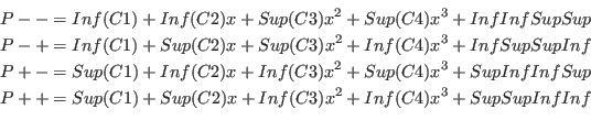
For a polynomial
 the four Kharitonov polynomials are:
The following procedure allows to determine if a polynomial has a real root
within a given range:
int Kharitonov(int Degree,
       INTERVAL_VECTOR (* TheCoeff)(double a,INTERVAL_VECTOR &),
       int (* Solve_Poly)(double *, int *,double *),
       INTERVAL_VECTOR &Input)
where:
- Degree: the degree of the polynomial
- TheCoeff: a procedure that allows to compute the
interval coefficients of the polynomial at a point a (i.e. the
coefficients of the polynomial
 )
)
- Solve_Poly: a procedure that compute the real part
of the roots of a
polynomial. It takes as argument the coefficients of the polynomial, a
pointer to an integer that is initially the degree of the polynomial
and the real roots are stored in the last argument. This
procedure returns the number of roots or -1 if the computation
has failed. ALIAS provides as possible procedure
ALIAS_Solve_Poly_PR.
- Input: the range for the root
Note that there exists an ALIAS-Maple procedure that uses this
procedure to generate a simplification procedure, see the ALIAS-Maple
manual.
Let  and the Gerschgorin circles defined as the set of
 such that:
The roots of the characteristic polynomial are enclosed in the union of
the  . Furthermore if a circle has no intersection with the other
circles, then this circle contains one root of the polynomial. This
allow for a fast determination of bounds for the real roots of the
polynomial.
. Furthermore if a circle has no intersection with the other
circles, then this circle contains one root of the polynomial. This
allow for a fast determination of bounds for the real roots of the
polynomial.
It is possible to get these bounds by using the procedure:
int Gerschgorin(INTERVAL_MATRIX &A,int Size, int Type, INTERVAL &Bound)
where:
- A: the matrix
- Size: the dimension of the matrix
- Type: 0 if the matrix is not available,
2 if the matrix is symmetrical, 1 otherwise
- Bound: all the roots will be enclosed in this interval
the procedure returns 1 if it has been possible to compute Bound.
A more complete procedure allows to get all the Gerschgorin circles
and eventually to adjust an interval that is supposed to contain the
roots of the polynomial:
int Gerschgorin_Simplification(INTERVAL_MATRIX &A,int Size,int Type,
                       INTERVAL &Input,INTERVAL_VECTOR &Circle)
The arguments are the same than the previous procedure
except for Input which is the interval
supposed to contain roots of the polynomial and Circle which
contain the projection of the Gerschgorin circle on the real axis.
This procedure returns:
- -1: Input does not contain a root of the polynomial
- 0: no change in Input
- 1: Input has been improved and the return value gives
the number of distinct circles
Cassini ovals
The Cassini ovals are another method to determine a bound for the
eigenvalues of a matrix.
Let and the Cassini ovals defined as the set of
such that:
Column based Cassini ovals may also be defined.
The roots of the characteristic polynomial are enclosed in the union of
the row-based and column-based  . Although more complicate to
calculate the bounds obtained with the Cassini ovals are usually
tighter than the bounds obtained with the Gerschgorin circles.
. Although more complicate to
calculate the bounds obtained with the Cassini ovals are usually
tighter than the bounds obtained with the Gerschgorin circles.
The Cassini bounds may be obtained with the procedure:
int Cassini_Simplification(INTERVAL_MATRIX &A,int Size,
                  int Type_Matrix, INTERVAL &Input)
where
- A: the matrix
- Size: the dimension of the matrix
- Type: 0 if the matrix is not available,
2 if the matrix is symmetrical, 1 otherwise
- Input: an estimation of the bounds of the roots
The procedure will return -1 if there is no intersection between Input and the Cassini bounds, 1 if there Input has been
improved, 0 otherwise.
This procedure may also be called with:
int Cassini_Simplification(int (* TheMatrix)(INTERVAL_VECTOR &, INTERVAL_MATRIX &),
      INTERVAL_VECTOR &Param,int Size, int Type_Matrix, INTERVAL &Input)
where TheMatrix is a procedure that compute the elements of the
matrix according to the interval value of the parameters Param.
Routh
The Routh algorithm allows to calculate
the number of roots with positive real part of a polynomial being given
the coefficients of the
polynomial. It is implemented as:
int Routh(int Degree,double *Coeff)
that returns the number of roots with positive real part or -1 if it
has not been possible to compute the Routh table (because the first
element of a row of the Routh table is close to 0).
A similar algorithm allows to deal with polynomial with interval
coefficients:
INTERVAL Routh(int Degree,INTERVAL_VECTOR &Coeff)
This algorithm returns in its interval:
- -1,-1
- : the Routh table cannot be computed
- a,a+1
- : there is at least a roots with positive real part but
the exact number of roots with positive real part cannot be calculated
- a,a
- : there is exactly a roots with positive real part
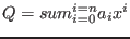
A similar procedure may be used when the coefficients are functions of
parameters:
INTERVAL Routh(int Degree,INTERVAL_VECTOR (* TheCoeff)(int,int,INTERVAL_VECTOR &),
               INTERVAL_VECTOR &Input)
where:
- TheCoeff: a procedure that allow to calculate the
coefficients being given the range for the parameters. It returns a
Degree+1 interval vector. The two first integers l1, l2 of the
procedure allows one to specify which coefficients are calculated. For
example if V=TheCoeff(1,5,Input), then V(1..5) will be the
first 5 coefficients of the polynomial and if V=TheCoeff(1,Degree+1,Input), then all the coefficients of the
polynomial will be available in V
- Input: the intervals for the parameter
If the derivatives of the coefficients with respect to the parameters
are known an even better procedure will be:
INTERVAL Routh(int Degree,INTERVAL_VECTOR (*TheCoeff)(int,int,INTERVAL_VECTOR &),
               INTERVAL_MATRIX (* TheCoeffG)(int,int,INTERVAL_VECTOR &),
               INTERVAL_VECTOR &Input)
where TheCoeffG is a procedure that allow to compute the
derivatives of the coefficients with respect to the parameters (see
note 2.4.2.2). This procedure allows to a certain amount to
take into account the dependency between the coefficients.
Note also that the procedure Routh of ALIAS-Maple allows an even
better calculation of the Routh table when dealing with parametric
polynomials as the elements of the Routh table are calculated
symbolically.
Weyl filter
Let  be a polynomial and be maxroot the maximal modulus of
the root of . From we may derive a the unitary polynomial
be a polynomial and be maxroot the maximal modulus of
the root of . From we may derive a the unitary polynomial  such that the
roots of have a modulus lower or equal to 1 and if
such that the
roots of have a modulus lower or equal to 1 and if  is a root
of then maxroot is a root of .
is a root
of then maxroot is a root of .
Let
 which may also be written as
 where
where  is some fixed point.
Let a range ![$[a,b]$](img608.png) for
for  and let
  be the mid point of the
range. We consider the square in the complex plane centered at
and whose edge length is
be the mid point of the
range. We consider the square in the complex plane centered at
and whose edge length is  . Let
. Let  be the length of the
half-diagonal of this square.
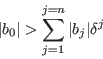
If
be the length of the
half-diagonal of this square.
If
then the polynomial has no root in the square [1].
This procedure may be used for univariate polynomial, with polynomial
with interval coefficients or with parametric poynomial. For example
it is very efficient for solging the Wilkinson polynomial.
The Weyl filter is implemented to manage univariate polynomial (with
numerical or interval coefficients) or parametric polynomial.
A basic tool of this filter is
int Weyl_Filter_Utility(int Degree, double maxroot,
                      INTERVAL_VECTOR &b,INTERVAL_VECTOR &Input)
where Input(1) is the range for the polynom variable and b
the  coefficients.
A more general implementation is
coefficients.
A more general implementation is
int Weyl_Filter(int Degree, INTERVAL_VECTOR &Coeff,double maxroot,
                int (* GetB)(int,INTERVAL_VECTOR &,INTERVAL &,INTERVAL_VECTOR &),
		INTERVAL_VECTOR &Input)
Here GetB is a procedure that calculates the
coefficients. Its arguments are the degree of the polynomial, its
coefficients, and the coefficients. It should return 1 if
the calculation has been successfull, 0 otherwise. An example of such
procedure is Derive_Polynomial_Expansion.
Degree is the degree of the polynomial, Coeff its
coefficients and Input(1) is the range for the polynomial
unknown.
This procedure has several variants:
int Weyl_Filter(int Degree, INTERVAL_VECTOR &Coeff,double max_root,
                INTERVAL_VECTOR &Input)
here the GetB procedure will be Derive_Polynomial_Expansion.
In
int Weyl_Filter(int Degree, INTERVAL_VECTOR &Coeff,
                INTERVAL_VECTOR &Input)
here the GetB procedure will be Derive_Polynomial_Expansion and maxroot will be computed by
an ALIAS procedure.
The same procedure will be used in
int Weyl_Filter(int Degree, INTERVAL_VECTOR &Coeff,
                int (* GetB)(int,INTERVAL_VECTOR &,INTERVAL &,INTERVAL_VECTOR &),
                INTERVAL_VECTOR &Input)
In some cases it may be difficult to obtain the analytical form of the
coefficients of the characteristic polynomial of a matrix. The
following procedure allows to compute these coefficients even if the
matrix is an interval matrix:
INTERVAL_VECTOR Coeff_CharPoly(int Size,INTERVAL_MATRIX &A)
where Size is the dimension of the matrix and A the
matrix. This procedures returns the coefficients in an interval vector
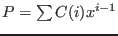
 and the polynomial is
 .
.


 Next: Linear algebra
Up: ALIAS-C++
Previous: Analyzing univariate polynomials
Next: Linear algebra
Up: ALIAS-C++
Previous: Analyzing univariate polynomials