Currents for shape representation

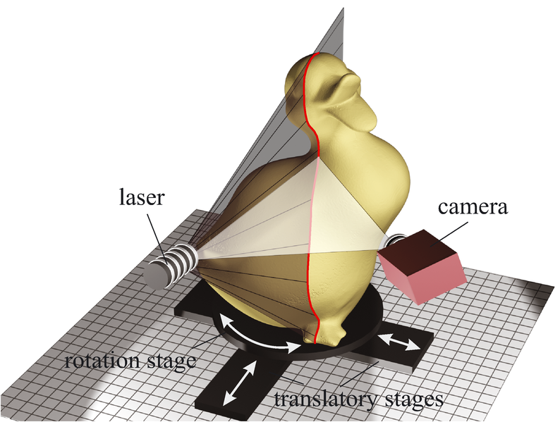
Currents are used to represent the shapes ⁱ and the residuals ϵⁱ of the forward model. Before going into the mathematical details, let consider a simple example. In the recent years, 3D scanners have been developed to digitalise 3D objects. These machines acquire the geometry of an object by probing its surface with laser beams. 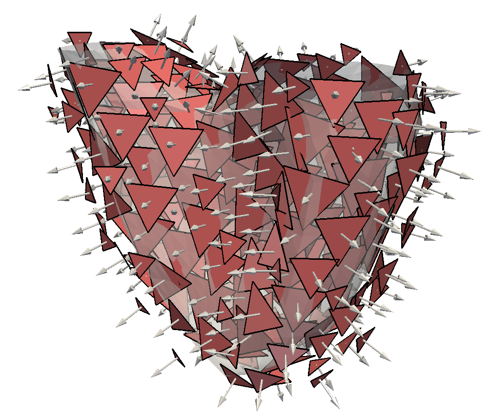The diffraction of the beams on the surface is captured by cameras and the resulting signal is used to reconstruct the virtual object. Likewise, currents characterise shapes by probing them using varying vector fields ω ∈ W , like virtual laser beams. The shape is characterised by how it integrates these vector fields (Figure 1).

Figure 1: 3D scanners digitalise 3D objects by probing their shape using varying laser beams (left panel). Currents function in the same way, they characterise a shape by probing it using varying vector fields (right panel)

Mathematically, a current is a continuous linear mapping _W (ω) from a vector space W to ℝ, i.e. it is an application that integrates vector fields. The current of a surface is the flux of a test vector field ω ∈ W across that surface. The shape of the surface S is uniquely characterised by the variations of the flux as the test vector field varies. The core element that makes this framework possible is to choose the vector space of the test vector fields W as the vector space generated by a Gaussian kernel K_W (,) = exp(-∥ -∥²∕λ_W ²) (W is a reproducible kernel Hilbert space (r.k.h.s.)). W is the dense span of basis vector fields of the form ω() = K_W (,), where the vectors are given and fixed at the spatial positions . The kernel K_W defines an inner product in W that can be easily computed by < ω(.),ν(.) > _W =< K_W (.,),K_W (.,) > _W = ^T K_W (,), where ω(.) = K_W (.,) and ν(.) = K_W (.,) are two vector fields of W . A consequence of these properties is that the space of currents W^*, which is the dual of W , is the dense span of the dual representations of the basis vectors ω(.), called Dirac delta currents δ(ω) and defined by:

(1)

Intuitively, a Dirac delta current is an infinitesimal vector that is concentrated at the spatial position . In that way, the current of a surface S can be decomposed into an infinite set of Dirac delta currents defined at each point of the surface and orientated along the surface normal. In our application, the surfaces are represented by discrete triangulated meshes. Their current representation is therefore given by the finite sum:

(2)

where _k are the barycentres of the mesh faces and _k their normal (Figure 2). The vector field ω dual of the current (ω) is the spatial convolution of every normal vector _k with the kernel K_W , ω() = ∑_kK_W (,_k)_k. In [1], the authors propose an efficient greedy algorithm to approximate the current representation of a surface by a minimal yet optimal set of Dirac delta currents (Figure 2). Computational complexity is further decreased by using FFT-based convolution techniques to compute the kernel convolutions.

Original Shape (1476 delta currents)	Compressed Shape (281 delta currents)

Figure 2: Dirac delta currents of a triangulated meshes are the normal vectors of every face, centred at the face barycentres. A greedy algorithm reduces the amount of delta currents needed to represent the shape while preserving the accuracy of the representation.

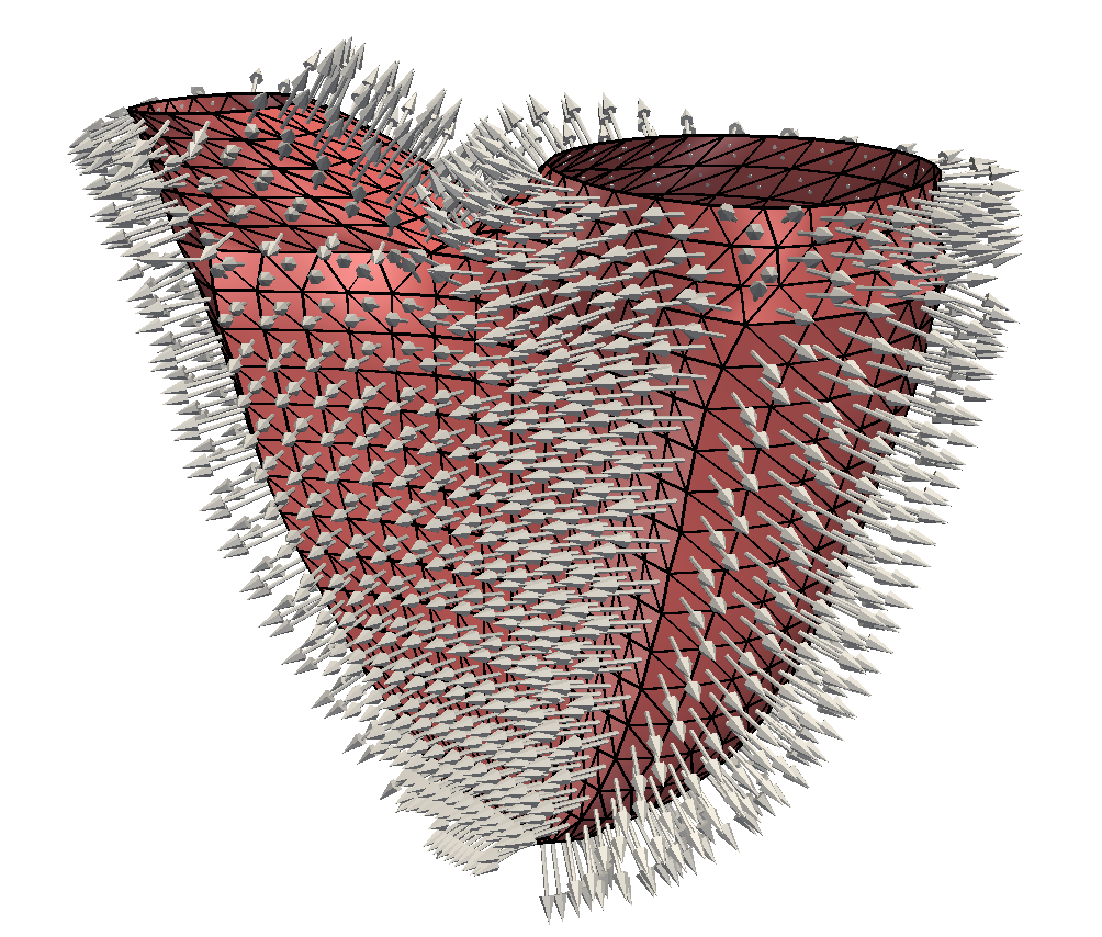As currents are linear applications, they define a vector space on shapes. The sum of two currents is the union of their Dirac delta currents, i.e. the union of the two surfaces. Likewise, scaling a current amounts to scaling the amplitude of the Dirac delta currents. By construction, the space of currents W^* is equipped with the inner-product < δ(ω),δ(ω) > _W^* =< K_W (,.),K_W (,.) > _W = ^T K_W (,). The distance between two shapes can therefore be computed as the norm of the difference of their currents. The space of currents thus enables us to compute mean, standard deviations and other descriptive statistics on shapes. Similarly, Gaussian variables in the space of currents can be defined. In practice, we place at each point _p of a 3D grid embedding the shape a random vector _p that follows a normal distribution.

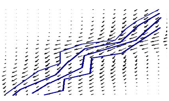
The width λ_W of the kernel K_W controls the resolution of the current representation. The larger λ_W , the coarser the resolution and the less “accurate” the representation. This parameter thus controls the level of shape details we want to study. As it is illustrated in Figure 3, small λ_W values enable capturing little differences between surfaces, whereas large λ_W discard them.

A)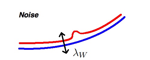

B)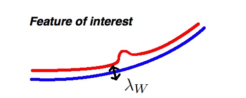

Figure 3: The size of the kernel K_W enables choosing the level of details of the current representation. Large λ_W discards subtle shape features (A) that would be recovered using smaller λ_W (B) (Images courtesy of S. Durrleman)

References

[1]    S. Durrleman, X. Pennec, A. Trouvé, and N. Ayache, “Statistical models on sets of curves and surfaces based on currents,” Medical Image Analysis, vol. 13, pp. 793–808, Oct. 2009.