La page de J-P. Merlet

J-P. Merlet home page

La page Présentation de HEPHAISTOS

HEPHAISTOS home page

La page "Présentation" de l'INRIA

INRIA home page

Subsections

• Introduction
• Finding bounds on the roots
  • First Cauchy theorem
    • Mathematical background
    • Implementation
    • Example
  • Second Cauchy theorem
    • Mathematical background
    • Implementation
    • Example
  • Third Cauchy theorem
    • Mathematical background
    • Implementation
  • Lagrange-MacLaurin theorem
    • Mathematical background
    • Implementation
    • Example
  • Laguerre method
    • Mathematical background
    • Implementation
    • Example
  • Laguerre second method
    • Mathematical background
    • Implementation
  • Newton method
    • Mathematical background
    • Implementation
  • Newton theorem
    • Mathematical background
    • Implementation
  • Joyal bounds
    • Mathematical background
    • Implementation
  • Pellet method
    • Mathematical background
    • Implementation
  • Global implementation
    • Example
  • Kantorovitch theorem
    • Implementation
    • Example
  
  
• Bounds on the product and sum of roots
  • Newton relations
    • Mathematical background
  • Implementation
  • Viète relations
    • Mathematical background
  • Implementation
  
  
• Maximum number of real roots
• Number of real roots
  • Descartes Lemma
    • Mathematical background
    • Implementation
  • Budan-Fourier method
    • Mathematical background
    • Implementation
    • Example
  • Sturm method
    • Mathematical background
    • Implementation
    • Example
  • Du Gua-Huat-Euler theorem
    • Mathematical background
    • Implementation
  
  
• Separation between the roots
  • Rump theorem
    • Mathematical background
    • Implementation
    • Example
  
  
• Analyzing the real roots
• Analyzing the real part of the roots
• Utilities
  • Addition of two polynomials
  • Multiplication of two polynomials
  • Evaluation of a polynomial
    • Evaluation in centered form
    • Safe evaluation of a polynomial
  • Sign of a polynomial
    • Implementation
  • Derivative of a polynomial
  • Euclidian division
  • Expansion of $(x-a)^n$
  • Centered form
  • Unitary polynomial
  • Safe evaluation of a vector

Analyzing univariate polynomials

Introduction

In this chapter we intend to determine some information on the roots of an univariate polynomial without solving it. A polynomial is defined by the list of its coefficient ordered along increasing power in a data structure of type VECTOR. For most of the procedures defined in the sequel the coefficients may also intervals, in which case the data structure is of type INTERVAL_VECTOR (this type of polynomial will be called interval polynomial).

Finding bounds on the roots

First Cauchy theorem

Mathematical background

Let $P(x)$ be an univariate polynomial of degree $n$:

$$P(x)= a_n x^n + a_{n-1} x^{n-1}+.....a_0=0$$

with $a_0a_n \not=0$. Let

$$A= max\{\mid a_{n-1}\mid ,\mid a_{n-2}\mid ,...,\mid a_0\mid... ...ime=max\{\mid a_n\mid ,\mid a_{n-1}\mid ,.....,\mid a_1\mid \}$$

Then the modulus of any root $x_k$ of $P(x)=0$ verify:

$$\frac{1}{1+\frac{A^\prime}{\mid a_0\mid }}<\mid x_k\mid < 1 + \frac{A}{\mid a_n\mid }$$

Implementation

This procedure is implemented as:

 
int Cauchy_First_Bound_Interval(int Degree,VECTOR &Coeff,INTERVAL &Bound);

with:

• Degree: degree of the polynomial
• Coeff: the Degree+1 coefficients of the polynomial in increasing degree
• Bound: the interval on the absolute value of the roots

This procedure returns 0 if Degree=0, Coeff(1)=0 or Coeff(Degree+1)=0 and Degree=1. On success the return code is 1. There is also an implementation for interval polynomial:

 
int Cauchy_First_Bound_Interval(int Degree,INTERVAL_VECTOR &Coeff,INTERVAL &Bound);

This procedure returns an interval $(\underline{Bound},\overline{Bound})$ such that for any polynomial in the set and for any root $x$ of this polynomial $\underline{Bound} \le \vert x\vert \le \overline{Bound}$. A failure code of 0 is returned if Coeff(1) or Coeff(Degree+1) contains 0 or if Degree=0. On success the returned code is 1.

Example

Let $P=x^3-x^2+2x-3$ and the procedure:

 
Coeff(1)= -3;Coeff(2)=2;Coeff(3)=-1;Coeff(4)=1;
Num=Cauchy_First_Bound_Interval(3,Coeff,Bound);

Coeff_App(1)= INTERVAL(-3.1,-2.9);Coeff_App(2)=INTERVAL(1.9,2.1);
Coeff_App(3)=INTERVAL(-1.1,-0.9);Coeff_App(4)=INTERVAL(0.9,1.1);
Num=Cauchy_First_Bound_Interval(3,Coeff_App,Bound);

In the first case the procedure find that the absolute value of the roots lie in [0.6,4] while in the second case the range is [0.58,4.44444].

Second Cauchy theorem

Mathematical background

Let $P(x)$ be an univariate polynomial of degree $n$:

$$P(x)= x^n + a_{1} x^{n-1}+.....a_n=0$$

with $a_n \not=0$. Let $a_{m_1},a_{m_2},\ldots$ with $m_1>m_2>\ldots$ the $k$ strictly negative coefficients of $P$. Then all the positive real roots of $P$ verify [13]:

$$x \le {\rm Max}\{ (k\vert a_{m_1}\vert)^{1/m_1},(k\vert a_{m_2}\vert)^{1/m_2},\ldots\}$$

Note that if $k=0$ all the roots are negative according to Descartes Lemma (see section 5.5.1).

Implementation

This procedure is implemented as:

 
int Cauchy_Second_Bound_Interval(int Degree,VECTOR &Coeff,double *Bound);

with:

• Degree: degree of the polynomial
• Coeff: the Degree+1 coefficients of the polynomial in increasing degree
• bound: the upper bound of the positive roots

This procedure returns 0 if the method cannot be applied because Degree=0 or Degree=1 and Coeff(2)=0. On success the return code is 1. It is also possible to determine the lower bound of the positive roots using:

 
int Cauchy_Second_Bound_Inverse_Interval(int Degree,VECTOR &Coeff,double *Bound);

This procedure fail and returns 0 if Degree=0, Degree=1 and Coeff(2)=0 or Coeff(1)=0. There is also an implementation for interval polynomial:

 
int Cauchy_Second_Bound_Interval(int Degree,INTERVAL_VECTOR &Coeff,INTERVAL Bound);

This procedure will return a failure code of 0 if Degree=0, Degree=1 and Coeff(2) contain 0, or if Coeff(Degree+1) contains 0. In that case if Bound=[a,b], then for all polynomials in the set the positive roots are all lower than b while for some polynomial in the set the roots are lower than a. Equivalently we have:

 
int Cauchy_Second_Bound_Inverse_Interval(int Degree,INTERVAL_VECTOR &Coeff,INTERVAL Bound);

In that case if Bound=[a,b], then for all polynomials in the set the positive roots are all lower than a while for some polynomial in the set the roots are lower than b.

A global procedure enable to get at the same time the upper and lower bound of the positive roots:

 
int Cauchy_Second_Bound_Interval(int Degree,VECTOR &Coeff,INTERVAL &Bound);
int Cauchy_Second_Bound_Interval(int Degree,INTERVAL_VECTOR &Coeff,
                           INTERVAL &Lower,INTERVAL &Upper);

In the latter case the interval lower bound is in Lower and the interval upper bound in Upper. It is also possible to determine the lower bound of the negative roots using the procedures:

 
int Cauchy_Second_Bound_Negative_Interval(int Degree,VECTOR &Coeff,double *Bound);
int Cauchy_Second_Bound_Negative_Interval(int Degree,INTERVAL_VECTOR &Coeff,INTERVAL &Bound);

while the upper bound of the negative roots can be determined using:

 
int Cauchy_Second_Bound_Negative_Inverse_Interval(int Degree,VECTOR &Coeff,double *Bound);
int Cauchy_Second_Bound_Negative_Inverse_Interval(int
Degree,INTERVAL_VECTOR &Coeff,
                  INTERVAL &Bound);

Both the upper and lower bound of the negative roots can be found using:

 
int Cauchy_Second_Bound_Negative_Interval(int Degree,VECTOR &Coeff,INTERVAL &Bound);
int Cauchy_Second_Bound_Negative_Interval(int Degree,INTERVAL_VECTOR &Coeff,
                                 INTERVAL &Lower,INTERVAL &Upper);

Example

Let $P=x^3-x^2+2x-3$ and the procedure:

 
Coeff(1)= -3;Coeff(2)=2;Coeff(3)=-1;Coeff(4)=1;
Num=Cauchy_Second_Bound_Interval(3,Coeff,&bound);
Coeff_App(1)= INTERVAL(-3.1,-2.9);Coeff_App(2)=INTERVAL(1.9,2.1);
Coeff_App(3)=INTERVAL(-1.1,-0.9);Coeff_App(4)=INTERVAL(0.9,1.1);
Num=Cauchy_Second_Bound_Interval(3,Coeff_App,Bound);

In the first case we find that all the roots are lower than 2 and in the second that the roots have bounds [2.44444,2.44444]. If we have used the lower bound procedures we will have found that all the roots are positive.

Third Cauchy theorem

Mathematical background

This procedure calculates a bound for the absolute value of the roots of the polynomial, see Handbook of numerical analysis, Ciarlet, Lions, Volume 3.

Implementation

 
int Cauchy_Third_Bound_Interval(int Degree,INTERVAL_VECTOR &Coeff,INTERVAL &Bound)

Coeff[1] cannot be 0. The procedure:

 
int Cauchy_All_Bound_Interval(int Degree,INTERVAL_VECTOR &Coeff,
                             INTERVAL &Bound)

will return the result of a successive application of the first and third Cauchy bounds.

Lagrange-MacLaurin theorem

Mathematical background

Let $P(x)$ be an univariate polynomial of degree $n$:

$$P(x)= a_0 x^n + a_{1} x^{n-1}+.....a_n=0$$

Assume $a_0>0$ and let $a_k$ ($k\ge 1$) be the first negative coefficients of $P(x)$ (if $P(x)$ has no negative coefficients then there is no positive real root).

The upper bound $M$ of the value of the positive real root is:

$$M=1+ \sqrt[k]{\frac{B}{a_0}}$$

where $B$ is the greatest absolute value of the negative coefficients of $P(x)$ ,[3],[13].

If we define:

$$P(y)=a_n y^n+ a_{n-1}y^{n-1}+.....+a_0$$

Then the upper bound of the positive real roots of $P(y)$ is the lower bound $m$ of the positive real root of $P(x)$. Consequently if $k$ and $B$ are computed for the polynomial $P(y)$ then

$$m=\frac{1}{1+\sqrt[n-k]{\frac{B}{a_n}}}$$

Implementation

This procedures is implemented as:

 
int MacLaurin_Bound_Interval(int Degree,VECTOR &Coeff,double *Bound);

with:

• Degree: degree of the polynomial
• Coeff: the Degree+1 coefficients of the polynomial in increasing degree
• bound: the upper bound of the positive roots

This procedure fail and returns 0 if Degree=0, Degree=1 and Coeff(2)=0 and if Coeff(Degree+1)=0.

On success the return code is 1. There is also a procedure for the interval polynomial:

 
int MacLaurin_Bound_Interval(int Degree,INTERVAL_VECTOR &Coeff,INTERVAL Bound);

This procedure fail and returns 0 if Degree=0, Degree=1 and $0 \in$Coeff(2) and if $0 \in$Coeff(Degree+1). In that case if Bound=[a,b], then for all polynomials in the set the roots are all lower than b while for some polynomial in the set the roots are lower than a.

It is also possible to determine the lower bound of the positive roots using the procedures:

 
int MacLaurin_Bound_Inverse_Interval(int Degree,VECTOR &Coeff,double *Bound);
int MacLaurin_Bound_Inverse_Interval(int Degree,INTERVAL_VECTOR &Coeff,INTERVAL &Bound);

In the later case if Bound=[a,b], then for all polynomials in the set the roots are all lower than a while for some polynomial in the set the roots are lower than b. To get directly both lower and upper bound of the positive roots you may use:

 
int MacLaurin_Bound_Interval(int Degree,VECTOR &Coeff,INTERVAL &Bound)
int MacLaurin_Bound_Interval(int Degree,INTERVAL_VECTOR &Coeff,INTERVAL &Lower, INTERVAL &Upper)

In the latter case the interval lower bound is in Lower and the interval upper bound in Upper.

It is also possible to determine the lower bound of the negative roots using the procedures:

 
int MacLaurin_Bound_Negative_Interval(int Degree,VECTOR &Coeff,double *Bound);
int MacLaurin_Bound_Negative_Interval(int Degree,INTERVAL_VECTOR &Coeff,INTERVAL &Bound);

Similarly it is possible to determine the upper bound of the negative roots using the procedures:

 
int MacLaurin_Bound_Negative_Inverse_Interval(int Degree,VECTOR &Coeff,double *Bound);
int MacLaurin_Bound_Negative_Inverse_Interval(int Degree,
                          INTERVAL_VECTOR &Coeff,INTERVAL &Bound);

To get directly both lower and upper bound of the negative roots you may use:

 
int MacLaurin_Bound_Negative_Interval(int Degree,VECTOR &Coeff,INTERVAL &Bound)
int MacLaurin_Bound_Negative_Interval(int Degree,INTERVAL_VECTOR &Coeff,
                              INTERVAL &Lower, INTERVAL &Upper)

Example

Let $P=x^3-x^2+2x-3$ and the procedure:

 
Coeff(1)= -3;Coeff(2)=2;Coeff(3)=-1;Coeff(4)=1;
Num=MacLaurin_Bound_Interval(3,Coeff,&bound);
Coeff_App(1)= INTERVAL(-3.1,-2.9);Coeff_App(2)=INTERVAL(1.9,2.1);
Coeff_App(3)=INTERVAL(-1.1,-0.9);Coeff_App(4)=INTERVAL(0.9,1.1);
Num=MacLaurin_Bound_Interval(3,Coeff_App,Bound);

In the first case we find that all the roots are lower than 4 and in the second that the roots have bounds [4.44444,4.44444]. If we have used the lower bound procedures we will have found that all the roots are greater than -1.

Laguerre method

Mathematical background

Let $P(x)$ be an univariate polynomial of degree $n$:

$$P(x)= a_0 x^n + a_{1} x^{n-1}+.....a_n=0$$

with $a_0a_n \not=0$, $a_0>0$. Let's define the sequence :

$$f_0=a_0, f_1=xf_0+a_1, \ldots,f_i =xf_{i-1}+a_i,\ldots,f_n=f_{n-1}+a_n=P$$

If it exists a real $c$ such that $f_i(c)\ge 0$ for all $i$ in [0,$n$], then $P(x)>0$ for all $x>c$. Consequently all the roots of $P$ are lower than $c$ [13]. To find $c$ the following scheme can be used:

1. let $c$ be such that $f_1(c) \ge 0$
2. let $k$ the smallest integer such that either $k=n+1$ or $k\le n$ and $f_k(c) \le 0$
3. if $k\le n$ then substitute $c$ by $c^\prime$ such that $f_k(c^\prime) \ge 0$ and go to 2
4. return $c$

A consequence of Laguerre theorem is that the best bound cannot be lower than $-a_1/a_0$.

Implementation

This procedure is able to give upper and lower bound on the value of the roots. In the implementation we define $c$ as the smallest real which satisfy $f_1(c) \ge 0$. If we find $k$ such that $f_k(c) \le 0$, then we increase $c$ by a given positive value sens and start again. We limit the number of iteration of the scheme by giving a maximal value for the number of iteration:

 
int Laguerre_Bound_Interval(int Degree,VECTOR &Coeff,double sens,int MaxIter,double *bound);

with:

• Degree: degree of the polynomial
• Coeff: the Degree+1 coefficients of the polynomial in increasing degree
• sens: a positive real indicating the increase of $c$ in the scheme
• MaxIter: the maximum number of iteration. If this number is exceeded the procedure returns 0.
• bound: the upper value of the real root

This procedure fail and returns 0 if Degree=0, Coeff(1)=0, if Coeff(Degree+1)=0 and if the number of iteration exceed MaxIter. On success the return code is 1. Note that the bound given by Laguerre (assuming that Coeff(Degree+1) is positive) cannot be lower than -Coeff(Degree)/Coeff(Degree+1).

The lower bound of the root may be determined by:

 
int Laguerre_Bound_Inverse_Interval(int Degree,VECTOR &Coeff1,double amp_sens,
                      int MaxIter,double *bound);

We have also a procedure which determine upper and lower bound for the real roots:

 
int Laguerre_Bound_Interval(int Degree,VECTOR &Coeff,double sens,int MaxIter,INTERVAL &Bound);

All the real roots lie within Bound. We may also use this procedure for interval polynomial:

 
int Laguerre_Bound_Interval(int Degree,INTERVAL_VECTOR &Coeff,double sens,
                              int MaxIter,INTERVAL &Bound);

This procedure fail and returns 0 if Degree=0, $0 \in$ Coeff(1), if $0 \in$Coeff(Degree+1) and if the number of iteration exceed MaxIter. If Bound=[a,b], then the real roots of all the polynomial in the set are lower than b and for some polynomial in the set the roots may be lower than a. A similar procedure exists for upper and lower bound.

 
int Laguerre_Bound_Interval(int Degree,INTERVAL_VECTOR &Coeff,double sens,
                        int MaxIter,INTERVAL &Lower,INTERVAL &Upper);

In that case Upper=[a,b] will be such that value of all roots of any polynomial within the set is lower than b, while for some polynomial they will be lower than a. On the other hand Lower=[a,b] will be such that the value of all roots of any polynomial within the set is greater than a, while for some polynomial they will be greater than b.

Example

The procedure:

 
Coeff(1)= -3;Coeff(2)=2;Coeff(3)=-1;Coeff(4)=1;
Num=Laguerre_Bound_Interval(3,Coeff,0.1,50,Bound);
Coeff_App(1)= INTERVAL(-3.1,-2.9);Coeff_App(2)=INTERVAL(1.9,2.1);
Coeff_App(3)=INTERVAL(-1.1,-0.9);Coeff_App(4)=INTERVAL(0.9,1.1);
Num=Laguerre_Bound_Interval(3,Coeff_App,0.1,50,Lower,Upper);

leads to Bound=[1.15385,1.3], Lower=[1.08209,1.40271], Upper=[1.21818,1.52222].

Laguerre second method

Mathematical background

Let $P(x)$ be an univariate polynomial of degree $n$:

$$P(x)= x^n + a_{1} x^{n-1}+.....a_n=0$$

Assume that $P$ has $n$ real roots. Then [23] all roots are contained in the interval whose end-point are given by the two solutions of the quadratic equation:

$$nx^2+2a_1x+[2(n-1)a_2-(n-2)a_1^2]=0$$

Implementation

This procedure enable to determine upper and lower bound on the roots of a polynomial if all the roots are real. In the implementation we check if all the roots of the polynomial are real using Huat theorem (see section 5.5.4) and if the answer is positive we determine the bounds. The syntax is:

 
int Laguerre_Second_Bound_Interval(int Degree,VECTOR &Coeff,INTERVAL &Bound);

with:

• Degree: degree of the polynomial
• Coeff: the Degree+1 coefficients of the polynomial in increasing degree
• Bound: upper and lower bound on the roots

On success the return code is 1 while the return code is 0 if the Degree is lower than 2. A similar algorithm exists for interval polynomial:

 
int Laguerre_Second_Bound_Interval(int Degree,
      INTERVAL_VECTOR &Coeff,INTERVAL &Lower,INTERVAL &Upper);

In that case Upper=[a,b] will be such that the maximal value of all roots of any polynomial within the set is lower than b, while for some polynomial they will be lower than a. On the other hand Lower=[a,b] will be such that the minimal value of all roots of any polynomial within the set is greater than a, while for some polynomial they will be greater than b.

Newton method

Mathematical background

Let $P(x)$ be an univariate polynomial of degree $n$:

$$P(x)= a_0 x^n + a_{1} x^{n-1}+.....a_n=0$$

with $a_0a_n \not=0$, $a_0>0$. Newton theorem state that if it exists $c$ such that $P(c)>0$ and for all the derivative $P^{(i)}$ of $P$, with $i \in [1,n]$, then $c$ is an upper bound of the positive roots of $P$. To find $c$ the following scheme can be used:

1. let $c$ be such that $P^{(n-1)}(c) \ge 0$
2. let $k$ the smallest integer such that either $k=n+1$ or $k\le n$ and $P^{(n-k)}(c) \le 0$
3. if $k\le n$ then substitute $c$ by $c^\prime$ such that $P^{n-k)}(c^\prime) \ge 0$ and go to 2
4. return $c$

A consequence of Newton theorem is that the best bound cannot be lower than $-a_1/(a_0 n)$.

Implementation

This procedure is able to give upper and lower bound on the value of the roots.

In the implementation we define $c$ as the smallest real which satisfy $P^{(n-1)}(c) \ge 0$. If we find $k$ such that $P^{(n-k)}(c) \le 0$, then we increase $c$ by a given positive value sens and start again. We limit the number of iteration of the scheme by giving a maximal value for the number of iteration:

 
int Newton_Bound_Interval(int Degree,VECTOR &Coeff1,double amp_sens,int MaxIter,double *bound);

with:

• Degree: degree of the polynomial
• Coeff: the Degree+1 coefficients of the polynomial in increasing degree
• sens: a positive real indicating the increase of $c$ in the scheme
• MaxIter: the maximum number of iteration. If this number is exceeded the procedure returns 0.
• bound: the upper value of the real root

This procedure fail and returns 0 if Degree=0, Coeff(1)=0, if Coeff(Degree+1)=0 and if the number of iteration exceed MaxIter. On success the return code is 1. Note that the bound given by Newton (assuming that Coeff(Degree+1) is positive) cannot be lower than -Coeff(Degree)/(Degree Coeff(Degree+1)). The lower bound of the root may be determined by:

 
int Newton_Bound_Inverse_Interval(int Degree,VECTOR &Coeff1,double amp_sens,
                      int MaxIter,double *bound);

We have also a procedure which determine upper and lower bound for the real roots:

 
int Newton_Bound_Interval(int Degree,VECTOR &Coeff1,double amp_sens,
                         int MaxIter,INTERVAL &Bound);

All the real roots lie within Bound. We may also use this procedure for interval polynomial:

 
int Newton_Bound_Interval(int Degree,INTERVAL_VECTOR &Coeff,double sens,
                              int MaxIter,INTERVAL &Bound);

This procedure fail and returns 0 if Degree=0, $0 \in$ Coeff(1), if $0 \in$Coeff(Degree+1) and if the number of iteration exceed MaxIter. If Bound=[a,b], then the real roots of all the polynomial in the set are lower than b and for some polynomial in the set the roots may be lower than a. A similar procedure exists for upper and lower bound.

 
int Newton_Bound_Interval(int Degree,INTERVAL_VECTOR &Coeff,double sens,
                        int MaxIter,INTERVAL &Lower,INTERVAL &Upper);

In that case Upper=[a,b] will be such that value of all roots of any polynomial within the set is lower than b, while for some polynomial they will be lower than a. On the other hand Lower=[a,b] will be such that the value of all roots of any polynomial within the set is greater than a, while for some polynomial they will be greater than b.

Newton theorem

Mathematical background

Let $P(x)$ be an univariate polynomial of degree $n$:

$$P(x)= a_0 x^n + a_{1} x^{n-1}+.....a_n=0$$

with $n$ real roots. The roots $x$ of $P$ are such that [4]:

$$x^2 <\left(\frac{a_1}{a_0} \right)^2-2 \left(\frac{a_2}{a_0}\right)$$

Implementation

This procedure is able to give an upper bound on the absolute value of the roots as soon as all the roots are real (this is checked using Huat theorem, section 5.5.4). The syntax is:

 
int Newton_Second_Bound_Interval(int Degree,VECTOR &Coeff,double *bound);

with:

• Degree: degree of the polynomial
• Coeff: the Degree+1 coefficients of the polynomial in increasing degree
• bound: upper bound on the absolute value of the roots

The procedure returns 0 if Degree=0 or Coeff(Degree+1)=0, 1 otherwise. We may also compute a lower bound on the absolute value of the root by using:

 
int Newton_Second_Bound_Inverse_Interval(int Degree,VECTOR &Coeff,double *bound);

An upper and lower bound on the absolute value of the roots may be compute by:

 
int Newton_Second_Bound_Interval(int Degree,VECTOR &Coeff,INTERVAL &Bound);

In that case if Bound=[a,b] we have for all root $x$: a$\le \vert x\vert \le$ b.

Similar procedures exist for interval polynomial:

 
int Newton_Second_Bound_Interval(int Degree,INTERVAL_VECTOR &Coeff,INTERVAL &Bound);
int Newton_Second_Bound_Inverse_Interval(int Degree,INTERVAL_VECTOR &Coeff,INTERVAL &Bound);
int Newton_Second_Bound_Interval(int Degree,INTERVAL_VECTOR &Coeff,INTERVAL &L, INTERVAL &U);

where

• Bound: upper or lower bound on the absolute value of the root of the polynomials
• L,U: if L=[a,b] then the absolute value of the roots of any polynomial in the set is greater than a while some polynomial have root greater than b. Conversely if U=[a,b] the absolute value of the roots of any polynomial in the set is lower than b while some polynomial have root lower than a.

Joyal bounds

Mathematical background

Let a polynomial whose interval coefficients have a fixed sign. Let $a_n$ be the leading coefficient such that $a_n=1$. We define the sequence $A_1=\vert a_{n-1}a_0\vert$, $A_2=\vert a_{n-1}a_1-a0\vert$, $A_j=\vert a_{n-1}a_j-a_{j-1}\vert$. If $A$ is the largest upper bound of the sequence $A_j$, then the modulus $\rho$ of the roots of the polynomial is lower or equal to $(1+\sqrt{1+4A})/2$.

Implementation

 
int Joyal_Bound_Interval(int Degre,INTERVAL_VECTOR &Coeff,INTERVAL
&Bound)

returns in Bound an upper bound of the modulus of the roots of the polynomial of degree Degre and interval coefficients Coeff. The procedure returns 0 if $a_n$ is not equal to 1, 1 otherwise.

Pellet method

Mathematical background

Let $f=a_n x^n+\ldots+a_0$ be a polynomial and let $f_p= \vert a_n\vert x^n+\ldots+\vert a_{p+1}x^{p+1}\vert-\vert a_p\vert x^p-\ldots-\vert a_0\vert$ be the associated polynomial. If $f_p$ has two positive roots $\beta>\alpha$, then $f$ has exactly $p$ roots in the disk $\vert x\vert<\alpha$ and no roots in the domain $\alpha <\vert x\vert<\beta$.

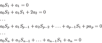
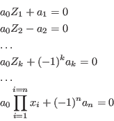
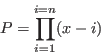
Now assume that we have calculated the coefficients of the polynomial $f(x+a+R)=Q(X)$ where $a, R$ are known quantities. If we determine a $Q_p$ polynomial that has 2 positive roots $a_1,a_2$ in the range $[0,R]$, then $Q(x)$ has roots in the disk $\vert X\vert<a_1<R$. Hence the absolute value of the real part of the roots is bounded by $a_1$. As $x=X-a-R$ we get that the real part $R_p$ of the root satisfies $-a_1+a+R\le R_p<a_1+a+R$. As $R>a_1$ this shows that $f$ has roots whose real part is greater than $a$.

Implementation

 
int Pellet(int Degre,INTERVAL_VECTOR &Coeff,double R)

where Degre is the degree of the polynomial, Coeff are the coefficients of the polynomial $f(x+a+R)$. This procedure returns 1 if roots whose real part is greater than $a$.

Global implementation

The above algorithms have been regrouped in two procedures, one for determining the bound on the positive roots, the other for the negative roots:

 
int Global_Positive_Bound_Interval(int Degree,VECTOR &Coeff,INTERVAL &Bound);
int Global_Negative_Bound_Interval(int Degree,VECTOR &Coeff,INTERVAL &Bound);

with:

• Degree: degree of the polynomial
• Coeff: the Degree+1 coefficients of the polynomial in increasing degree
• Bound: the bound on the positive or negative roots

For the positive root if Bound=[a,b] and b=0, then there is no positive root. Similarly for the negative root is a=0, then there is no negative root. The procedure returns 0 in case of failure which correspond to the failure of all the previous algorithms, 1 in case of success. Note that for Laguerre and Newton method the maximum number of iteration is defined by the global variable Max_Iter_Laguerre_Interval fixed by default to 1000. The step size is defined as:

• if a bound $B$ have been previously determined, then the step size is fixed to $B/30$ except if the global variable Step_Laguerre_Interval has been defined to be a double not equal to 0, in which case this variable is used as the step size.
• if a bound as not been determined the step size is fixed to 1 except if the global variable
  Step_Laguerre_Interval has been defined to be a double not equal to 0, in which case this variable is used as the step size.
• if the step if lower than the global variable Min_Step_Laguerre_Interval (which is 0.1 by default) the step is substituted by Min_Step_Laguerre_Interval

Similar procedure exist for interval polynomial:

 
int Global_Positive_Bound_Interval(int Degree,INTERVAL_VECTOR &Coeff,
                           INTERVAL &Lower,INTERVAL &Upper);
int Global_Negative_Bound_Interval(int Degree,INTERVAL_VECTOR &Coeff,
                           INTERVAL &Lower,INTERVAL &Upper);

where Lower is an interval on the lower bound: for positive roots and if Lower=[a,b] then the roots of any polynomial in the set is greater than a while some polynomial have root greater than b. Conversely if Upper=[a,b] the roots of any polynomial in the set is lower than b while some polynomial have root lower than a.

Both procedures for real roots have been regrouped in

 
void ALIAS_Find_Bound_Polynom(int Degree,
         INTERVAL_VECTOR (* TheCoeff)(INTERVAL_VECTOR &), 
         INTERVAL_VECTOR &PALL,INTERVAL &Space, INTERVAL &Bound)

where

• PALL: the first component is the bound for the real roots the polynomial while the following are the value of the parameters for which the bounds will be obtained
• Space: a default bound for the real roots; may be used to indicate that we are looking only for bounds on the positive or negative real roots by specifying a positive or a negative lower bound
• Bound: bounds for the real roots

Example

An interesting example is given by:

 
Coeff_App(1)= INTERVAL(-3.1,-2.9);Coeff_App(2)=INTERVAL(1.9,2.1);
Coeff_App(3)=INTERVAL(-1.1,-0.9);Coeff_App(4)=INTERVAL(0.9,1.1);
Num=Global_Positive_Bound_Interval(3,Coeff_App,Lower,Upper);

which leads to Lower=[1.1487,1.42957], Upper=[1.15224,1.43049].

The above procedure may give some sharp bounds. For example consider the Wilkinson polynomial of order 22 (which has as roots 1,2,$\ldots$,21,22) we get 0 negative roots while the positive roots are bounded by [0.790447,22.1087].

The test program Test_Bound_UP enable to test the bound procedures for any polynomial. This program take as first argument the name of a file giving the coefficients of the polynomial by increasing power of the variable. The program will print the bounds determined by all the previous procedures and then the bounds determined using the global implementation. Then the same treatment will be applied on the interval polynomial whose coefficients are intervals centered at the coefficients find in the file with a width of 0.2

Kantorovitch theorem

The mathematical background of Kantorovitch has been explained in section 3.1.2. This method may determine an interval on the unknown in which there is an unique solution, toward which Newton method will converge (see section 2.9).

Implementation

The syntax of the algorithm is:

 
int Kantorovitch(int Degree,VECTOR &Coeff,REAL Input,double *eps)

with

• Degree: degree of the polynomial
• Coeff: coefficients of the polynomial ordered along increasing degree
• Input: center of the interval in which an unique solution occur
• eps: half width of the solution interval

If this procedure returns 1, then there is an unique solution in the interval [Input-eps,Input+eps]. There is also an implementation of Kantorovitch theorem for interval polynomial:

 
int Kantorovitch(int Degree,INTERVAL_VECTOR &Coeff,REAL Input,double *eps)

If this procedure returns 1, then any polynomial in the set of interval polynomial has an unique solution in the interval [Input-eps,Input+eps]. There is also an implementation which take into account rounding errors:

 
int Kantorovitch_Fast_Safe(int Degree,INTERVAL_VECTOR &Coeff,REAL Input,double *eps)

in which "safe" interval value of the coefficients have been pre-computed.

Example

Let $P=x^3-x^2+2x-3$, Input be 1.2 and the procedure:

 
Coeff(1)= -3;Coeff(2)=2;Coeff(3)=-1;Coeff(4)=1;
Num=Kantorovitch(3,Coeff,1.2,&eps);
Coeff_App(1)= INTERVAL(-3.1,-2.9);Coeff_App(2)=INTERVAL(1.9,2.1);
Coeff_App(3)=INTERVAL(-1.1,-0.9);Coeff_App(4)=INTERVAL(0.9,1.1);
Num=Kantorovitch(3,Coeff_App,1.2,&eps);

In the first case Kantorovitch returns 1 and has determined that there is an unique solution in the interval [1.04082,1.35918]. Using Newton method we find the root 1.27568220371567 with residue 2.80147904874184e-10. For the interval polynomial Kantorovitch returns also 1 and find an unique solution in [1.05718,1.34282].

Bounds on the product and sum of roots

Newton relations

Mathematical background

Let $P(x)$ be an univariate polynomial of degree $n$:

$$P(x)= a_0 x^n + a_{1} x^{n-1}+.....a_n=0$$

and $x_1,\ldots,x_n$ the real and complex roots of $P$. Let define $S_p$ as

$$S_p=\sum_{i =1}^{i =n} x_i^p$$

We have [4]:

$$\begin{eqnarray*} && a_0S_1+a_1=0\\ && a_0S_2+a_1S_1+2a_2=0\\ && \ldots\\ && ... ..._p=0\\ &&\ldots\\ && a_0S_n+a_1S_{n-1}+\ldots+a_{n-1}S_1+a_n=0 \end{eqnarray*}$$

Implementation

Let $x_i$ be the $n$ roots (either complex or real) of a polynomial of degree $n$. Let $S_p$ be:

$$S_p=\sum_{i =1}^{i =n} x_i^p$$

This procedure enable to compute the $n$ elements $S_1,\ldots,S_n$. The syntax is:

 
VECTOR SumN_Polynomial_Interval(int Degree,VECTOR &Coeff)

with:

• Degree: degree of the polynomial
• Coeff: coefficients of the polynomial ordered along increasing degree

This procedure returns 0 if the leading coefficient is equal to 0, 1 otherwise. There is an equivalent procedure for interval polynomial:

 
INTERVAL_VECTOR SumN_Polynomial_Interval(int Degree,INTERVAL_VECTOR &Coeff)

which returns intervals including the $S_p$. This procedure returns 0 if 0 is included in the leading interval.

Viète relations

Mathematical background

Let $P(x)$ be an univariate polynomial of degree $n$:

$$P(x)= a_0 x^n + a_{1} x^{n-1}+.....a_n=0$$

and $x_1,\ldots,x_n$ the real and complex roots of $P$. Let define $Z_p$ as:

$$Z_p= \sum_{i<j<\ldots<k,i =1,\ldots,n} x_ix_j\ldots x_k$$

We have [4]:

$$\begin{eqnarray*} && a_0Z_1+a_1=0\\ && a_0Z_2-a_2=0\\ && \ldots\\ && a_0Z_k+(-1)^ka_k=0\\ &&\ldots\\ && a_0\prod_{i =1}^{i =n}x_i+(-1)^na_n=0 \end{eqnarray*}$$

Implementation

Let $x_i$ be the $n$ roots (either complex or real) of a polynomial of degree $n$. Let $Z_p$ be:

$$Z_p= \sum_{i<j<\ldots<k,i =1,\ldots,n} x_ix_j\ldots x_k$$

This procedure enable to compute the $n$ elements $Z_1,\ldots,Z_n$ ($Z_1$ is the sum of the roots, $Z_n$ the product of the roots). The syntax is:

 
VECTOR ProdN_Polynomial_Interval(int Degree,VECTOR &Coeff)

with:

• Degree: degree of the polynomial
• Coeff: coefficients of the polynomial ordered along increasing degree

This procedure returns 0 if the leading coefficient is equal to 0, 1 otherwise. There is an equivalent procedure for interval polynomial:

 
INTERVAL_VECTOR ProdN_Polynomial_Interval(int Degree,INTERVAL_VECTOR &Coeff)

which returns intervals including the $Z_p$. This procedure returns 0 if 0 is included in the leading interval.

Maximum number of real roots

Number of real roots

Descartes Lemma

Mathematical background

Let $P$ the polynomial:

$$P=a_0+a_1x+\ldots+a_nx^n$$

with $a_0a_n \not=0$. Let the sequence $\{a_0,a_1,\ldots,a_n\}$ and the $n$ the number of change of sign in this sequence. Then the number of positive real roots, counted with their order of multiplicity is equal to $n-2k$ with $k\in [0,n/2]$ [13].

Implementation

The syntax of the procedure is:

 
INT Descartes_Lemma_Interval(int Degree,VECTOR &Coeff)

with:

• Degree: degree of the polynomial
• Coeff: the Degree+1 coefficients of the polynomial in increasing degree

This procedure returns the number of positive real roots up to an even number. If the procedure returns $m$ the number of positive roots is $m-2k$ with $k\in[0,m/2]$.

There is an implementation of this method for interval polynomial. Here it is necessary to introduce an additional parameter to indicate the confidence we have in the result. The procedure is implemented as:

 
INT Descartes_Lemma_Interval(int Degree,INTERVAL_VECTOR &Coeff,int *Confidence);

Confidence is a quality index:

• 1: the result is exact, for all polynomials in the set the number of positive real roots is $m-2k$
• $\le 0$: the number of positive real roots for all the polynomials in the set is $\le m$

Similar algorithms for negative roots are available:

 
INT Descartes_Lemma_Negative_Interval(int Degree,VECTOR &Coeff)
INT Descartes_Lemma_Negative_Interval(int Degree,INTERVAL_VECTOR &Coeff,int *Confidence)

Budan-Fourier method

Mathematical background

Budan-Fourier algorithm is a simple method which enable to determine easily some information on the number of root of a given univariate polynomial within a given interval. Let $P$ the polynomial:

$$P=a_0+a_1x+\ldots+a_nx^n$$

and $P^{(n)}$ its n-th derivative. Let the interval $(\underline{x},\overline{x})$ the interval in which we are looking for roots. We assume that $P(\underline{x}) \not=0$, $P(\overline{x}) \not=0$ and $a_0 \not= 0$. We construct the sequence $L=\{P(\underline{x}),P^{(1)}(\underline{x}),\ldots,P^{(n)}(\underline{x})\}$ from which we exclude the 0 element. Similarly we construct the sequence $U=\{P(\overline{x}),P^{(1)}(\overline{x}),\ldots,P^{(n)}(\overline{x})\}$ (a special treatment has to be applied for the zero element of $U$, see [13]). Let $\underline{N}$ the number of change of sign in $L$ and $\overline{N}$ the number of change of sign in $U$. Then the number of real roots of $P$ in $(\underline{x},\overline{x})$, counted with their order of multiplicity, is $\underline{N}-\overline{N}$ or lower than this number by an even number.

Implementation

This procedure is used to determine the number of real roots in a given interval, up to an even number. The syntax of the procedure is:

 
INT Budan_Fourier_Interval(int Degree,VECTOR &Coeff,INTERVAL In)
INT Budan_Fourier_Interval(int Degree,INTEGER_VECTOR &Coeff,INTERVAL In)

with:

• Degree: degree of the polynomial
• Coeff: the Degree+1 coefficients of the polynomial in increasing degree, which may be REAL or INT
• In: the interval in which we are looking for the number of roots

If this procedure returns the integer $m \ge 0$, then the number of real roots in In is $m-2k$ with $k\in[0,m/2]$. A negative returns code indicate a failure of the algorithm:

• -1: $P(\underline{{\tt In}})=0$
• -2: $a_0=0$, the polynomial may be factored
• -3: $P(\overline{{\tt In}})=0$

This procedure may be used with polynomial whose coefficients are intervals. The syntax is:

 
INT Budan_Fourier_Interval(int Degree,INTERVAL_VECTOR &Coeff,INTERVAL In,int *Confidence)

where Confidence is a quality index for the result:

• 1: the result is exact, so if $m$ is the return code of the algorithm the number of reals roots of the interval polynomial is $m-2k$ with $k\in[0,m/2]$
• $\le 0$: if $m$ is the return code of the algorithm the number of reals roots of the interval polynomial is $\le m$

Due to rounding errors incorrect results may be returned by the previous procedures. A safer procedure is:

 
INT Budan_Fourier_Safe_Interval(int Degree,VECTOR &Coeff,
                                INTERVAL In,INTERVAL &NbRoot);

The procedure returns 1 in case of success and an interval for the number of roots. If NbRoot=[a,b], then if a =b the number of roots is either a,a-2,$\ldots$ and if a $\not=$ b the number of roots is lower than b. If "safe" value of the coefficients have been pre-computed you may use:

 
INT Budan_Fourier_Fast_Safe_Interval(int Degree,INTERVAL_VECTOR &Coeff,
                                     INTERVAL In,INTERVAL &NbRoot);

Another safe procedure is:

 
INT Budan_Fourier_Interval(int Degree,INTEGER_VECTOR &Coeff,int Inf,int Sup)

where the coefficients and the bounds are integers.

Example

Let $P=x^3-x^2+2x-3$, In be the interval [0,2] and the procedure:

 
Coeff(1)= -3;Coeff(2)=2;Coeff(3)=-1;Coeff(4)=1;
P=INTERVAL(0.0,2.0);
Num= Budan_Fourier_Interval(3,Coeff,P);

Num is 3 meaning that $P$ has either 3 or 1 roots in the interval. Now assume that we have an interval polynomial:

 
Coeff_App(1)= INTERVAL(-3.1,-2.9);
Coeff_App(2)=INTERVAL(1.9,2.1);
Coeff_App(3)=INTERVAL(-1.1,-0.9);
Coeff_App(4)=INTERVAL(0.9,1.1);
Num= Budan_Fourier_Interval(Degree,Coeff_App,P,&Confidence);

Num is also 3 with Confidence=1 meaning that the number of roots for any polynomial is either 3 or 1.

Sturm method

Mathematical background

Let a polynomial $P$ and define $f_0=P$, $f_1$ be the first derivative of $P$. Then define the sequence $f_i = -{\tt Rem}(f_{i-2},f_{i-1})$ where Rem is the remainder of the division of $f_{i-2}$ by $f_{i-1}$. If $n$ is the degree of $P$ the last element in the sequence will be $f_n$. Assume now that we are looking for the number of distinct roots of $P$ in the interval $[a,b]$ with $P(a)P(b)\not=0$. We build two sequences:

$$\{ f_0(a),f_1(a),\ldots,f_n(a)\}   \{ f_0(b),f_1(b),\ldots,f_n(b)\}$$

Let $n_0$ be the number of change of sign in the first sequence and $n_1$ be the number of change of sign in the second sequence. Then the number of distinct real roots of $P$ in the interval $[a,b]$ is $n_0-n_1$ [14] if $f_0(a)f_0(b)\not =0$. Note that a multiple roots count only for one root with this method.

The drawback of Sturm method is that the absolute value of the coefficients increase quickly when computing the sequence. Numerical rounding errors may then affect the result. The alternate method of Budan-Fourier (see section 5.5.2) is less sensitive to rounding errors although it provides less information than Sturm method.

Implementation

This procedure determines the number of real roots of an univariate polynomial in a given interval. It is implemented as:

 
int Sturm_Interval(int Degree,VECTOR &Coeff,INTERVAL &In);
int Sturm_Interval(int Degree,INTEGER_VECTOR &Coeff,INTERVAL &In);

• Degree: degree of the polynomial
• Coeff: the Degree+1 coefficients of the polynomial in increasing degree, either real or integers
• In: the interval in which we are looking for the number of roots

This procedure returns 0 or a positive number on success, this number being the number of roots of the polynomial in the interval. A return code of -1 means that either the polynomial is equal to 0, is equal to 0 at one of the extremity of the interval or has multiple roots. However Sturm method is sensitive to numerical rounding errors. For high degree polynomial it may be better to use the "safer" procedure:

 
int Sturm_Safe_Interval(int Degree,VECTOR &Coeff,INTERVAL &In,INTERVAL &NbRoot);

which returns 1 in case of success and an interval NbRoot which contain the number of roots. If NbRoot=[a,b], then if a =b the number of roots is a and if a $\not=$ b the number of roots is lower than b. Another safe procedure can be used if the coefficients are integers and the interval is also defined by integer numbers:

 
int Sturm_Interval(int Degree,INTEGER_VECTOR &Coeff,int Inf,int Sup);

This procedure will return -1 if all the coefficients are 0 and -2 if at some point of the process an integer larger than the largest machine integer is encountered (Not yet implemented).

Example

We use as example the Wilkinson polynomial of degree $n$ where $P$:

$$P= \prod_{i =1}^{i =n} (x-i)$$

and we are looking for roots in the interval [0.5,0.7] the procedure Sturm_Interval returns always 0 for order 4 to 20. But starting at order 9 the safe procedure returns [0,3] while the safe Budan-Fourier procedure still returns 0.

The test program Test_Nb_Root_Up enable to test Budan-Fourier and Sturm method on any polynomial whose coefficients are defined in a file, by increasing degree of the power of the unknown.

Du Gua-Huat-Euler theorem

Mathematical background

Let $P$ the polynomial:

$$P=a_0+a_1x+\ldots+a_nx^n$$

If all the roots of $P$ are real then [13]:

$$a_i ^2 \ge a_{i-1}a_{i+1}    {\rm for }  i \in [1,n]$$

Conversely if this relation does not hold for some $i$ (for example if a coefficient is 0 while its neighbor have same sign), then there are complex roots.

Implementation

This procedure enable to determine if the roots of a polynomial are all real. It is implemented in a safe way i.e. if they are numerical errors in the coefficients and if the procedure determine that all the roots are real the result is guaranteed. The syntax is:

 
int Huat_Polynomial_Interval(int Degree,VECTOR &Coeff);

with:

• Degree: degree of the polynomial
• Coeff: the Degree+1 coefficients of the polynomial in increasing degree

This procedure returns 1 if all the roots are real, 0 otherwise. There is a similar procedure for interval polynomial:

 
int Huat_Polynomial_Interval(int Degree,INTERVAL_VECTOR &Coeff);

This procedure will return 1 if all the polynomials in the set have their roots real, -1 if some polynomials in the set have all roots real but some others have complex roots and 0 if all the polynomials in the set have complex roots.

Separation between the roots

Rump theorem

Mathematical background

Let $P$ the polynomial:

$$P=a_0+a_1x+\ldots+a_nx^n$$

and let $\vert P\vert$ be:

$$\vert P\vert={\rm Max}_{i =0}^{i =n} \vert a_i\vert$$

The minimal distance $\Delta$ between the real roots of $P$ is such that [26]:

$$\Delta > \sqrt{\frac{8}{n^{n+2}}}\frac{1}{1+\vert P\vert^n}$$

Implementation

The procedure is able to determine a lower bound on the distance between two real roots of a polynomial:

 
int Min_Sep_Root_Interval(int Degree,VECTOR &Coeff,double &min);

with

• Degree: degree of the polynomial
• Coeff: the Degree+1 coefficients of the polynomial in increasing degree
• min: the lower bound on the distance between two real roots

Similarly an upper bound may be determined with:

 
int Max_Sep_Root_Interval(int Degree,VECTOR &Coeff,double &max);

while upper and lower bounds may be determined with:

 
int Bound_Sep_Root_Interval(int Degree,VECTOR &Coeff,INTERVAL &Bound);

There is also a procedure to determine a lower bound for interval polynomial:

 
int Min_Sep_Root_Interval(int Degree,INTERVAL_VECTOR &Coeff,INTERVAL &Lower);

If Lower=[a,b] then some polynomials in the set will have a minimal distance between the roots greater than b while all the polynomials in the set have a minimal distance greater than a.

Example

Clearly this formula give an underestimated value of the minimal distance between the roots. For example if we consider a Wilkinson polynomial of order 4 (which has therefore 1,2,3,4 as roots) we find that the minimal and maximal distance between the roots are bounded by [7.07107e-09,1.41421e+08].

Analyzing the real roots

The procedure

 
int ALIAS_Min_Max_Is_Root(int Degree,  
  int NbParameter,
  int HasInterval,
  INTERVAL_VECTOR (* TheCoeff)(INTERVAL_VECTOR &), 
  int Iteration,
  INTERVAL_VECTOR &Par,
  double *Root,
  int Type,
  int (* Solve_Poly)(double *, int *,double
*))

may be used to rest if a polynomial in a set may have as real root one of two pre-defined value.

• Degree: the degree of the polynomial
• NbParameter: the number of parameters that appear in the coefficient of the polynomial
• HasInterval: 1 if the coefficient include intervals not defined by parameters, 0 otherwise
• TheCoeff: a procedure to calculate the coefficients of the polynomial being given range for the parameters
• Iteration: the maximum number of box that may be used by the algorithm
• Par: the ranges for the parameters
• Root: we look for polynomial whose real part of the root is either Root[0] or Root[1]
• Type:
  • -1 : if in a box we have found a polynomial with a root lower than Root[0]; we look for a polynomial in the box whose real root is exactly Root[0]. If no such polynomial is found the box is eliminated
  • 1 : if in a box we have found a polynomial with a root greater than Root[1]; we look for a polynomial in the box whose real root is exactly Root[1]. If no such polynomial is found the box
  • 2: if in a box we have found a polynomial with a root greater than Root[1] and a polynomial with a real root greater than Root[0]; we look for a polynomial in the box whose real root is exactly Root[1] and a polynomial whose real root is exactly Root[0]. If no such polynomials are found the box is eliminated
  • 0: general case;
• Solve_Poly: a procedure to solve polynomial with double floating point coefficients. The first argument are the coefficients, the second the degree of the polynomial and the third the real roots

This procedure returns -1 if no polynomial with real root Root exist, 1 if such polynomial exist and 0 if the algorithm has not be able to determine such polynomial

Analyzing the real part of the roots

For some applications it may be interesting to determine if a polynomial in a set defined by a parametric polynomial has the real part of one of its roots equal to a pre-defined value. This may be done by using the procedure

 
int ALIAS_Is_Root_RealPart(int Degree,  
           int NbParameter,
           int HasInterval,
           INTERVAL_VECTOR (* TheCoeff)(INTERVAL_VECTOR &), 
           INTERVAL_VECTOR (* TheCoeffCentered)(INTERVAL_VECTOR&,double a), 
           int Iteration,
           INTERVAL_VECTOR &Par,
           double *Root,
           INTERVAL_VECTOR (* EvaluateComplex)(int,int,INTERVAL_VECTOR &),
           int (* Simp)(INTERVAL_VECTOR &))

where

• Degree: the degree of the polynomial
• NbParameter: the number of parameters that appear in the coefficient of the polynomial
• HasInterval: 1 if the coefficient include intervals not defined by parameters, 0 otherwise
• TheCoeff: a procedure to calculate the coefficients of the polynomial being given range for the parameters
• TheCoeffCentered: a procedure to calculate the coefficients of the polynomial $P(x+a)$
• Iteration: the maximum number of box that may be used by the algorithm
• Par: the ranges for the parameters
• Root: we look for polynomial whose real part of the root is either Root[0] or Root[1]
• EvaluateComplex: a procedure that returns 4 intervals. The input interval vector has dimension NbParameter+1 elements, the first one being the parameters, the last one being $b$. The procedure should evaluate $U=P(Root[0]+I b), V=P(Root[1]+I b)$ and should return the real part of $U$, the complex part of $U$, the real part of $V$ and the complex part of $V$
• Simp: an optional simplification procedure that returns -1 if the polynomials in a set cannot roots with real part equal to Root[0] or Root[1]

Utilities

Addition of two polynomials

The following procedures enable to add polynomials with real,interval or integer coefficients:

 
VECTOR Add_Polynomial_Interval(int n1,VECTOR &Coeff1,int n2,VECTOR &Coeff2);
INTERVAL_VECTOR Add_Polynomial_Interval(int n1,INTERVAL_VECTOR &Coeff1,
                  int n2,INTERVAL_VECTOR &Coeff2);
INTEGER_VECTOR Add_Polynomial_Interval(int n1,INTEGER_VECTOR &Coeff1,
      int n2,INTEGER_VECTOR &Coeff2);

with:

• ni: degree of the polynomial
• Coeffi: the coefficients of the polynomials in increasing degree

There is also a version which take into account rounding errors:

 
INTERVAL_VECTOR Add_Polynomial_Safe_Interval(int n1,VECTOR &Coeff1,int n2,VECTOR &Coeff2);

Multiplication of two polynomials

The following procedures returns the degree of the product of two polynomial either with real or integer coefficients:

 
int Degree_Product_Polynomial_Interval(int n1,VECTOR &Coeff1,int n2,VECTOR &Coeff2);
int Degree_Product_Polynomial_Interval(int n1,INTEGER_VECTOR &Coeff1,int n2,
      INTEGER_VECTOR &Coeff2);

Then you may use the following procedure to compute the product of polynomial either with real,integer or interval coefficients:

 
VECTOR Multiply_Polynomial_Interval(int n1,VECTOR &Coeff1,int n2,VECTOR &Coeff2);
INTEGER_VECTOR Multiply_Polynomial_Interval(int n1,INTEGER_VECTOR &Coeff1,
      int n2,INTEGER_VECTOR &Coeff2);
INTERVAL_VECTOR Multiply_Polynomial_Interval(int n1,INTERVAL_VECTOR &Coeff1,
      int n2,INTERVAL_VECTOR &Coeff2);

All these procedures return the coefficients of the product, the leading term being 0 only if one polynomial is equal to 0.

To take into account the rounding errors you may use:

 
INTERVAL_VECTOR Multiply_Polynomial_Safe_Interval(int n1,VECTOR &Coeff1,int n2,VECTOR &Coeff2);

Evaluation of a polynomial

The evaluation of a polynomial for a given value is implemented as:

 
REAL Evaluate_Polynomial_Interval(int Degree,VECTOR &Coeff,REAL P)
INTERVAL Evaluate_Polynomial_Interval(int Degree,INTERVAL_VECTOR &Coeff,REAL P)
INTERVAL Evaluate_Polynomial_Interval(int Degree,VECTOR &Coeff,INTERVAL P)
INTERVAL Evaluate_Polynomial_Interval(int Degree,INTERVAL_VECTOR &Coeff,INTERVAL P)
REAL Evaluate_Polynomial_Interval(int Degree,INTEGER_VECTOR &Coeff,REAL P);
int Evaluate_Polynomial_Interval(int Degree,INTEGER_VECTOR &Coeff,INT P);

with:

• Degree: degree of the polynomial
• Coeff: the Degree+1 coefficients (which can be REAL, INT or INTERVAL of the polynomial in increasing degree
• P: the point at which we want to compute the polynomial. It may be REAL, INT or INTERVAL.

These procedures enable to get:

• the value of a polynomial with REAL coefficients at a point
• the interval value of a polynomial with interval coefficients at a real point
• the interval value of a polynomial with REAL coefficients at for an interval value of the unknown. The first and second order derivative of the polynomial are used to get sharp bounds
• the interval value of a polynomial with interval coefficients for an interval value of the unknown. The first and second order derivative of the polynomial are used to get sharp bounds

Evaluation in centered form

The previous procedures may yield sometime to a bad evaluation of the polynomial. For example for the Wilkinson polynomial at order 15 the evaluation for 15.1 leads to 11977410100.791748046875, the correct value being 11977396665.006561033796551. The evaluation obtained when considering that the coefficients and the unknown are intervals is evidently correct and leads to the interval:

 
[11977379510.705810546875,11977410100.791748046875]

A better evaluation may be obtained if we use a centered form of the polynomial. Consider the polynomials:

$$\begin{eqnarray*} &&P=a_0+a_1x+\ldots+a_nx^n\\ &&P_1=b_0+b_1(x-c)+\ldots+b_n(x-c)^n \end{eqnarray*}$$

where $c$ is a real. For an appropriate choice of the $b_i$ we may have $P=P_1$ for all $x$. The procedures:

 
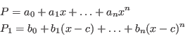
VECTOR Coeff_Polynomial_Centered_Interval(int Degree,VECTOR &Coeff,REAL P);
INTERVAL_VECTOR Coeff_Polynomial_Centered_Interval(int Degree,
                  INTERVAL_VECTOR &Coeff,REAL P);

enable to compute the $b_i$ for the centered form at P either for polynomial or interval polynomial. To take into account numerical errors you may use:

 
INTERVAL_VECTOR Coeff_Polynomial_Centered_Safe_Interval(int Degree,VECTOR &Coeff,REAL P);
INTERVAL_VECTOR Coeff_Polynomial_Centered_Fast_Safe_Interval(int Degree,
           INTERVAL_VECTOR &Coeff,REAL P);

which return safe value for the coefficients (in the second form we assume that you have pre-computed safe value for the coefficients of the polynomial using the procedure described in section 5.9.10).

Then we may use the procedures:

 
REAL Evaluate_Polynomial_Centered_Interval(int Degree,VECTOR &Coeff,REAL Center,REAL P);
INTERVAL Evaluate_Polynomial_Centered_Interval(int Degree,VECTOR &Coeff,INTERVAL P);
INTERVAL Evaluate_Polynomial_Centered_Interval(int Degree,INTERVAL_VECTOR &Coeff,
    REAL Center,REAL P);
INTERVAL Evaluate_Polynomial_Centered_Interval(int Degree,INTERVAL_VECTOR &Coeff,INTERVAL P);

These procedures return the evaluation of the polynomial at P using the centered form at Center or at the middle point of P if is an interval. For example for the Wilkinson polynomial at order 15 the evaluation for 15.1 using the centered form at 15 leads to 11977396665.00650787353516 which is largely better than the previous evaluation.

Safe evaluation of a polynomial

Due to the numerical error in the coefficients and in $x$ the evaluation of a polynomial at $x$ may be incorrect. The following procedures enable to compute an interval which is guaranteed to include the true value:

 
INTERVAL Evaluate_Polynomial_Safe_Interval(int Degree,VECTOR &Coeff,REAL P);
INTERVAL Evaluate_Polynomial_Safe_Interval(int Degree,VECTOR &Coeff,INTERVAL P);
INTERVAL Evaluate_Polynomial_Safe_Interval(int Degree,INTERVAL_VECTOR &Coeff,REAL P);
INTERVAL Evaluate_Polynomial_Safe_Interval(int Degree,INTERVAL_VECTOR &Coeff,INTERVAL P);

For example for the Wilkinson polynomial at order 15 the evaluation for 15.1 leads to the interval:

$$[11977320583.22778129577637,11977474081.67480659484863].$$

If "safe" intervals have been pre-computed (for example by using the procedure described in section 5.9.10) for the coefficients you may use:

 
INTERVAL Evaluate_Polynomial_Fast_Safe_Interval(int Degree,INTERVAL_VECTOR &Coeff,REAL P);
INTERVAL Evaluate_Polynomial_Fast_Safe_Interval(int Degree,INTERVAL_VECTOR &Coeff,INTERVAL P);

which are faster. If you want to use a centered form you may use:

 
INTERVAL Evaluate_Polynomial_Centered_Safe_Interval(int Degree,VECTOR &Coeff,REAL P);
INTERVAL Evaluate_Polynomial_Centered_Safe_Interval(int Degree,VECTOR &Coeff,INTERVAL P);
INTERVAL Evaluate_Polynomial_Centered_Fast_Safe_Interval(int Degree,
        INTERVAL_VECTOR &Coeff,REAL P);
INTERVAL Evaluate_Polynomial_Centered_Fast_Safe_Interval(int Degree,
       INTERVAL_VECTOR &Coeff,INTERVAL P);

in which the two last forms assume that you have pre-computed a safe value of the coefficients of the polynomial.

The evaluation of a polynomial with real coefficients at a complex point may be performed with:

INTERVAL_VECTOR Evaluate_Complex_Poly(int deg,
        INTERVAL_VECTOR &Coeff, INTERVAL &XR,INTERVAL &XI)

where XR is the real part of the point and XI its imaginary part. This procedure returns an interval vector whose first element is the real part of the evaluation and the second element its imaginary part.

Sign of a polynomial

This procedure is able to determine if the sign of a polynomial evaluated at a given point may be affected by numerical errors.

Implementation

 
int Sign_Polynomial_Interval(int Degree,VECTOR &Coeff,REAL P)
int Sign_Polynomial_Interval(int Degree,INTERVAL_VECTOR &Coeff,REAL P)
int Sign_Polynomial_Interval(int Degree,INTERVAL_VECTOR &Coeff,REAL P)
int Sign_Polynomial_Interval(int Degree,INTERVAL_VECTOR &Coeff,INTERVAL P)

with:

• Degree: degree of the polynomial
• Coeff: the Degree+1 coefficients (which can be REAL or INTERVAL of the polynomial in increasing degree
• P: the point or interval at which we want to compute the polynomial

This procedure returns 1 if the polynomial is positive, -1 if it is negative, 0 if it is 0 and 2 if the sign is either affected by numerical errors (if Coeff and P are REAL) or is not constant (if Coeff or P are INTERVAL_VECTOR).

Derivative of a polynomial

The derivatives of a polynomial may be computed using the procedures:

 
VECTOR Derivative_Polynomial_Interval(int Degree,VECTOR &Coeff)
INTEGER_VECTOR Derivative_Polynomial_Interval(int Degree,INTEGER_VECTOR &Coeff);
VECTOR Nth_Derivative_Polynomial_Interval(int Degree,VECTOR &Coeff,int n)

These procedures enable to get the coefficients of the first and n-th derivative of a polynomial defined by its REAL or INT coefficients.

Due to rounding errors there may be errors in the coefficients provided by the previous procedures. The procedure:

 
INTERVAL_VECTOR Derivative_Polynomial_Safe_Interval(int Degree,VECTOR &Coeff);

will return an INTERVAL_VECTOR (i.e. a set of intervals) which are guaranteed to include the true value of the coefficients of the derivative. A faster procedure may be used if "safe" interval values of the coefficients have been pre-computed:

 
INTERVAL_VECTOR Derivative_Polynomial_Fast_Safe_Interval(int Degree,INTERVAL_VECTOR &Coeff);

If we deal with polynomial with interval coefficients the following procedures may be used:

 
INTERVAL_VECTOR Derivative_Polynomial_Interval(int Degree,INTERVAL_VECTOR &Coeff)
INTERVAL_VECTOR Nth_Derivative_Polynomial_Interval(int Degree,
                                    INTERVAL_VECTOR &Coeff,int n)

Euclidian division

The procedure:

 
void ALIAS_Euclidian_Division(int Degree,INTERVAL_VECTOR &Coeff1,
     INTERVAL_VECTOR &Coeff2,INTERVAL &Residu,INTERVAL &a)

computes the division of the polynomial P with interval coefficients Coeff1 by x-a and returns the polynomial P1 with coefficients Coeff2 such that P=(x-a)P1+Residu

Another procedure that perform the same process if a is a double is

 
void Divide_Single(int Degree,INTERVAL_VECTOR &Coeff1,double a, 
                   INTERVAL_VECTOR &Coeff2, INTERVAL &Residu)

For dividing a polynomial $P$ by the product of polynomials of type $(x-a_1)(x-a_2)\ldots(x-a_n)$ so that

$$P(x)=(x-a_1)(x-a_2)\ldots(x-a_n)Q(x)+R(x)$$

and evaluating the polynomial under this form for some interval $X$ for $x$ you may use

 
INTERVAL Divide_Evaluate_Multiple(int Degree,INTERVAL_VECTOR &Coeff1,
                                  int n,double *a,INTERVAL_VECTOR &X)

where

• n: the number of terms $a_i$
• a: the value of $a_1,\ldots,a_n$

The interval returned by this procedure is the the interval evaluation of $P$ for $x$ having the the interval value $X(1)$.

For the Euclidian division by an arbitrary polynomial you may use

 
int Divide_Polynom(int Degree,INTERVAL_VECTOR &Coeff,int DegreeDivisor,
                   INTERVAL_VECTOR &CoeffDivisor,
		   INTERVAL_VECTOR &CoeffQuo, INTERVAL_VECTOR &CoeffRem)

The polynomial $P$ of degree Degree with cofficients Coeff will be divided by the polynomial $S$ of degree DegreeDivisor with coefficients CoeffDivisor so that the coefficient will be a polynomial $Q$ of degree Degree-DegreeDivisor with coefficients CoeffQuo with a reminder which is a polynomial of degree DegreeDivisor and coefficients CoeffRem. This procedure returns 0 if the division is not possible (the interval coefficient of the leading term of $S$ includes 0) or if the degree of $S$ is greater than the degree of $P$. If the division has been performed this procedure will return 1.

Note that Divide_Polynom and Divide_Evaluate_Multiple may be used to perform the deflation of an univariate polynomial as soon as approximate roots for the polynomial have been found. This may be useful to decrease the computation time for solving a polynomial or for numerically instable polynomial such as the Wilkinson polynomial. A combination of Rouche filtering and of deflation allows to solve Wilkinson polynomial of order 18, while the general solving procedure will fail starting at order 13.

A special Euclidian division is the division of a polynomial $P$ by its derivative. This can be done with

 
void Quotient_UP_Derivative(int Degree,VECTOR &Coeff,VECTOR &CoeffD,VECTOR &Quo,
                            VECTOR &Rem)

where $P$ has coefficients Coeff, its derivative CoeffD and the coefficient of the division is Quo (the quotient is a polynomial of degree 1) while the coefficients of the remainder are stored in Rem

Expansion of $(x-a)^n$

The coefficients of the expansion of the polynomial $(x-a)^n$ may be obtained with the procedure

 
INTERVAL_VECTOR Power_Polynomial(INTERVAL &a,int n)

which returns the coefficients

Centered form

Let $P=sum_{i=0}^{i=n} a_i x^i$ which may also be written as $sum_{i=0}^{i=n} b_i(x-a)^i$ where $a$ is some fixed or interval value. The coefficient $b_i$ may be calculated with the procedure

 
int Derive_Polynomial_Expansion(int n,INTERVAL_VECTOR &Coeff,INTERVAL &a,INTERVAL_VECTOR &B)

which returns 1 if the $b_i$ have been successfully calculated (0 otherwise). The coefficients of $P$ are Coeff and the $b_i$ are stored in B.

Unitary polynomial

Let $P$ be a polynomial and be maxroot the maximal modulus of the root of $P$. From $P$ we may derive a polynomial $Q$ such that the roots of $Q$ have a modulus lower or equal to 1 and if $w$ is a root of $Q$ then maxroot$w$ is a root of $P$. The calculation of the coefficients of $Q$ may be done with the procedure

 
int Unit_Polynom(int Degree,INTERVAL_VECTOR &Coeff,
                double maxroot,INTERVAL_VECTOR &CoeffU)

where Coeff are the coefficients of $P$ and CoeffU the coefficients of $Q$. This procedure returns 1 if the calculation has been successfull, 0 otherwise.

Safe evaluation of a vector

Let us consider a VECTOR: due to numerical rounding each element of this vector represent in fact an interval. The procedure:

 
INTERVAL_VECTOR Evaluate_Coeff_Safe_Interval(int n,VECTOR &Coeff);

with:

• n: size of the vector
• Coeff: the vector

returns an INTERVAL_VECTOR guaranteed to include the true value of the elements of the vector.

J-P. Merlet home page

La page Présentation de HEPHAISTOS

HEPHAISTOS home page

La page "Présentation" de l'INRIA

INRIA home page