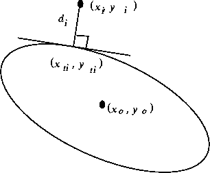
To overcome the problems with the algebraic distances, it is natural to replace them by the orthogonal distances which are invariant to transformations in Euclidean space and which do not exhibit the high curvature bias.
The orthogonal distance ![]() between a point
between a point ![]() and a
conic Q(x,y) is the Euclidean distance between
and a
conic Q(x,y) is the Euclidean distance between ![]() and the point
and the point
![]() in the conic whose tangent is orthogonal to the
line joining
in the conic whose tangent is orthogonal to the
line joining ![]() and
and ![]() (see fig:orth-dis).
(see fig:orth-dis).

Figure 2: Orthogonal distance of a point to a conic
Given n points ![]() (
( ![]() ), the orthogonal distance fitting is
to estimate the conic Q by minimizing the following function
), the orthogonal distance fitting is
to estimate the conic Q by minimizing the following function
However, as the expression of ![]() is very complicated (see below), an
iterative optimization procedure must be carried out. Many techniques are
readily available, including Gauss-Newton algorithm, Steepest Gradient
Descent, Levenberg-Marquardt procedure, and simplex method. A software
ODRPACK (written in Fortran) for weighted orthogonal distance regression is
domain public and is available from NETLIB (netlib@ornl.gov).
Initial guess of the conic parameters must be supplied, which can be obtained
using the techniques described in the last section.
is very complicated (see below), an
iterative optimization procedure must be carried out. Many techniques are
readily available, including Gauss-Newton algorithm, Steepest Gradient
Descent, Levenberg-Marquardt procedure, and simplex method. A software
ODRPACK (written in Fortran) for weighted orthogonal distance regression is
domain public and is available from NETLIB (netlib@ornl.gov).
Initial guess of the conic parameters must be supplied, which can be obtained
using the techniques described in the last section.
Let us now proceed to compute the orthogonal distance ![]() . The subscript i
will be omitted for clarity. Refer again to fig:orth-dis. The conic
is assumed to be described by
. The subscript i
will be omitted for clarity. Refer again to fig:orth-dis. The conic
is assumed to be described by
![]()
Point ![]() must satisfy the following two equations:
must satisfy the following two equations:
Equation (9) merely says the point ![]() is on the conic, while
(10) says that the tangent at
is on the conic, while
(10) says that the tangent at ![]() is orthogonal to the vector
is orthogonal to the vector
![]() .
.
Let ![]() and
and ![]() . From (9),
. From (9),
where ![]() . From (10),
. From (10),
![]()
Substituting the value of ![]() (11) in the above equation leads to the
following equation:
(11) in the above equation leads to the
following equation:
where

Squaring the above equation, we have
![]()
Rearranging the terms, we obtain an equation of degree four in ![]() :
:
where

The two or four real roots of (13) can be found in closed form. For one
solution ![]() , we can obtain
, we can obtain ![]() from (12), i.e.:
from (12), i.e.:
![]()
Thus, ![]() is computed from (11). Eventually comes the orthogonal
distance d, which is given by
is computed from (11). Eventually comes the orthogonal
distance d, which is given by
![]()
Note that we possibly have four solutions. Only the one which gives the smallest distance is the one we are seeking for.