import multipers as mp
import multipers.grids as mpg
import numpy as np
import gudhi as gd
import matplotlib.pyplot as plt
np.random.seed(2)
Custom multi-filtrations
Toy examples
This notebook will showcase how to use the multipers library core functions. As it relies on gudhi code, the syntax is almost the same.
The example we provide can be tweaked in different ways; don’t hesitate to read the functions documentations to figure out how to do so.
st = gd.SimplexTree() # usual gudhi simplextree
st.insert([0,1],1)
st.insert([1],0)
# converts the simplextree into a multiparameter simplextree
st_multi = mp.SimplexTreeMulti(st, num_parameters=2)
list(st_multi)
[(array([0, 1]), array([  1., -inf])),
 (array([0]), array([  1., -inf])),
 (array([1]), array([  0., -inf]))]
st = mp.SimplexTreeMulti(num_parameters=2) # multiparameter syntax
st.insert([0],[0,1])
st.insert([1],[1,0])
st.insert([0,1],[1,1])
list(st) # list of (simplex, filtration)
[(array([0, 1]), array([1., 1.])),
 (array([0]), array([0., 1.])),
 (array([1]), array([1., 0.]))]
Almost all methods of gudhi simplextree should work ootb on simplextreemultis, and some are reimplemented, e.g., make_filtration_non_decreasing, expand, edge_collapse.
Furthermore, some methods are removed, e.g., persistence, and are replaced by other topological invariants. For instance interval approximations, provided by MMA (wich comes itself with its own PyModule structure), or signed measures derived from the dimension vector of the module or the Euler characteristic.
mma_pymodule = mp.module_approximation(st)
mma_pymodule.plot(degree=0, box=[[0,0],[2,2]])
mma_pymodule[0].get_birth_list(), mma_pymodule[0].get_death_list() ## The coordinates of the red shape
([array([0., 1.]), array([1., 0.])], [array([inf, inf])])

The signed measure obtained by the degree 0 homology can be retrieved using
mp.signed_measure(st, degree=0)
((array([[0., 1.],
         [1., 0.],
         [1., 1.]]),
  array([ 1,  1, -1])),)
And the signed measure obtained via the euler characteristic (degree=None)
mp.signed_measure(st)
((array([[0., 1.],
         [1., 0.],
         [1., 1.]]),
  array([ 1,  1, -1], dtype=int32)),)
On point clouds
# Dataset
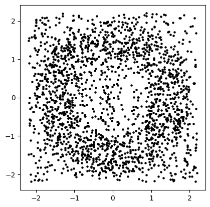
from multipers.data import noisy_annulus
X = noisy_annulus(n1=1000, n2=1000) # 1000 points on the annulus, 500 points on the square.
plt.scatter(X[:,0], X[:,1], s=5, c='k');plt.gca().set_aspect(1);
# Gudhi SimplexTree
st = gd.RipsComplex(points=X, sparse=.2).create_simplex_tree()
# SimplexTreeMulti, with 2 parameters
st = mp.SimplexTreeMulti(st, num_parameters=2)
st is now a SimplexTreeMulti, whose first parameter is a rips, and the second parameter is undefined.
Let’s fill the second parameter.
from multipers.ml.convolutions import KDE as KernelDensity
codensity = - KernelDensity(bandwidth=0.2).fit(X).score_samples(X)
# parameter = 1 is the second parameter as python starts with 0.
st.fill_lowerstar(codensity, parameter=1) # This fills the second parameter with the co-log-density
[KeOps] Warning : Cuda libraries were not detected on the system or could not be loaded ; using cpu only mode
<multipers.simplex_tree_multi.SimplexTreeMulti_Ff64 at 0x7fee6c0925f0>
Note that the KernelDensity is a (faster) reimplementation of sklearn’s KernelDensity, using PyKeops, which allows us to do automatic-differentiation.
Remark : A rips complex contains a lot of unnecessary edges, which can make the filtration grid prohibitly large; we will simplificate the simplextree, before computing this exact grid. This can be done using the collapse_edges method, which relies on filtration_domination.
print("Before edge collapses :", st.num_simplices)
st.collapse_edges(-2) # This should take less than 20s. -1 is for maximal "simple" collapses, -2 is for maximal "harder" collapses.
print("After edge collapses :", st.num_simplices)
st.expansion(2) # Be careful, we have to expand the dimension to 2 before computing degree 1 homology.
print("After expansion :", st.num_simplices)
Before edge collapses : 175216
After edge collapses : 9716
After expansion : 21250
Interval decomposition approximation
To get an idea of the shape of the module, we can compute first an approximation of it, using MMA.
mp.module_approximation(st).plot(degree=1) # Should take less than ~10 seconds depending on the seed
Signed Barcode Decompositions
Another interesting topological invariants are signed measures given by module decompositions. Unlike MMA, they heavily rely on computation on a fixed grid, so in order to significantly reduce the computational time, we can coarsen the multi-filtration before doing the computations. This can be done using the grid_squeeze method.
The easiest measure to compute on point cloud is the one given by the decomposition of the hilbert function, i.e., the pointwise dimension of the module.
st_coord = mp.SimplexTreeMulti(st) # We do a copy first (for later use), as this changes the filtration values.
st_coord = st_coord.grid_squeeze(grid_strategy="exact") # exact filtration
list(st_coord.get_simplices())[:3] # filtration values are now integers : the coordinates in that grid
[(array([  0, 104, 963]), array([4347, 1246], dtype=int32)),
 (array([   0,  104, 1020]), array([3449, 1216], dtype=int32)),
 (array([   0,  104, 1308]), array([2334, 1216], dtype=int32))]
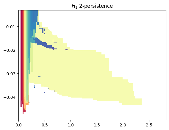
We can now compute the signed measure of degree 1 of this complex.
# The zero pad zeros out the grid, should take less than ~10s
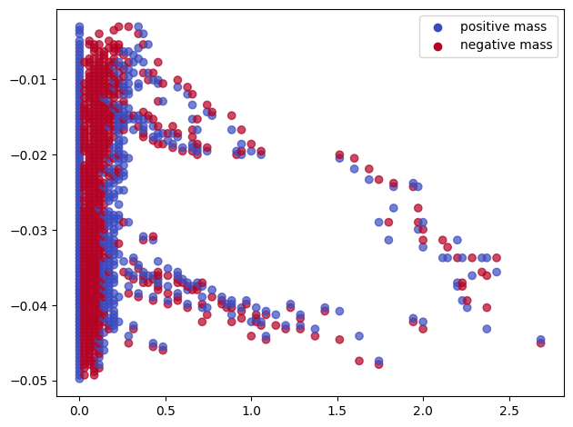
sm_hilbert = mp.signed_measure(st_coord,degrees=[1], plot=True, mass_default=None, invariant="hilbert")
Note that the Euler signed measure cannot be computed here (unless you have a lot of RAM), as one would need to do a st.expansion(#num_verticies) beforehand.
This is why we need to simplificate the original multi-filtration, by using a grid of lower resolution.
filtration_grid = mpg.compute_grid(st, strategy="regular", resolution=100)
[f.shape for f in filtration_grid] # filtrations of parameter 1 (radius) and 2 (codensity)
[(100,), (100,)]
st_coord = st.grid_squeeze(filtration_grid) # Squeezing simplificates the multi-filtration,  thus we can collapse edges again :)
st_coord.collapse_edges(-2) ## Warning because edge collapses only cares about dimensions 0 and 1. Mute with `ignore_warning`.
st_coord.expansion(st_coord.num_vertices)
st_coord.num_simplices
/tmp/ipykernel_179626/3288068986.py:2: UserWarning: This method ignores simplices of dimension > 1 !
  st_coord.collapse_edges(-2) ## Warning because edge collapses only cares about dimensions 0 and 1. Mute with `ignore_warning`.
40155
# should be instantaneous
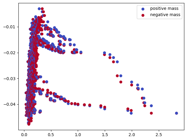
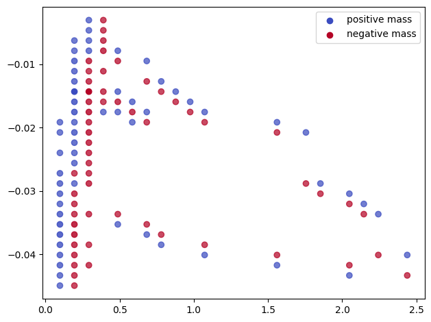
sm_euler = mp.signed_measure(st_coord,degree=None,plot=True) # degree=None automatically calls the euler invariant, and integers the hilbert invariant
Note. When simplifications (e.g. collapses) are not necessary, or not possible (e.g., not a clique complex) this grid coarsening can be directly called in the signed measure arguments:
mp.signed_measure(st, grid_strategy="regular", degree=1, resolution=30,plot=True); # The previous Hilbert signed measure, with a smaller grid
Finally, the measure given by the rank decomposition has an even worse scaling with the grid size, so we recommend decreasing the grid size before computing this measure.
## The rank invariant can be even slower to compute; it is in particular very affected by the resolution.
st_coord = st.grid_squeeze(grid_strategy="regular_closest", resolution=50) # Arguments for grid computation can also be provided instead of the grid
st_coord.collapse_edges(-2, ignore_warning=True)
sm_rank, = mp.signed_measure(st_coord,degrees=[1], invariant="rank")
sm_hilbert1 = mp.signed_measure(st_coord, degree=1, invariant="hilbert")
(pts, weights), = sm_hilbert1
hf, grid = mp.point_measure.integrate_measure(pts,weights, return_grid=True)
mp.plots.plot_surface(grid, hf, discrete_surface=True)
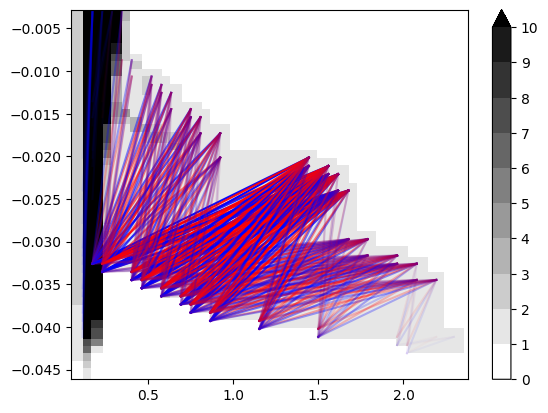
mp.plots.plot_signed_measure(sm_rank)
Signed Measure Vectorizations
Sliced Wasserstein
For the slicedwasserstein distances, and the convolutions of the signed measures, we recommend to use the already provided pipelines :
multipers.ml.multi.SignedMeasure2Convolutionmultipers.ml.multi.SignedMeasure2SlicedWassersteinDistance
Note that the second one needs signed measures of null mass. So set the zero_pad flag to True when using these pipelines.
from multipers.ml.signed_measures import SignedMeasure2Convolution, SignedMeasure2SlicedWassersteinDistance, SignedMeasureFormatter
[sm_hilbert, sm_euler] = SignedMeasureFormatter(normalize=True).fit_transform([sm_hilbert, sm_euler])
imgs = SignedMeasure2Convolution(plot=True,bandwidth=0.05, grid_strategy='regular', resolution=200).fit_transform([sm_hilbert, sm_euler])

Multi-critical multi-Filtrations
Note. This is still experimental, and interface is subject to changes.
Furthermore, no other library is compatible with multi-critical filtrations, so calling code that requires them will not work.
Check the simplextree with list(st) if necessary.
import multipers as mp
import numpy as np
Simply add the simplices multiple times! This can also seamlessly be converted to multi-critical slicers
st = mp.SimplexTreeMulti(num_parameters=2, kcritical=True, dtype = np.float64)
st.insert([0,1,2], [0,1])
st.insert([0,1,2], [1,0])
st.remove_maximal_simplex([0,1,2])
st.insert([0,1,2], [1,2])
st.insert([0,1,2], [2,1])
st.insert([0,1,2],[1.5,1.5])
st.insert([0,1,2], [2.5,.5])
st.insert([0,1,2], [.5,2.5])
list(st)
[(array([0, 1, 2]),
  [array([0.5, 2.5]),
   array([1., 2.]),
   array([1.5, 1.5]),
   array([2., 1.]),
   array([2.5, 0.5])]),
 (array([0, 1]), [array([0., 1.]), array([1., 0.])]),
 (array([0, 2]), [array([0., 1.]), array([1., 0.])]),
 (array([0]), [array([0., 1.]), array([1., 0.])]),
 (array([1, 2]), [array([0., 1.]), array([1., 0.])]),
 (array([1]), [array([0., 1.]), array([1., 0.])]),
 (array([2]), [array([0., 1.]), array([1., 0.])])]
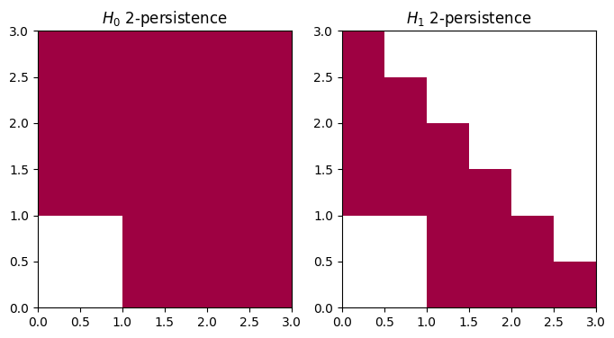
mp.module_approximation(st, box = [[0,0],[3,3]]).plot()