Point Cloud Optimization

import multipers as mp
from multipers.data import noisy_annulus, three_annulus
import multipers.ml.point_clouds as mmp
import multipers.ml.signed_measures as mms
import gudhi as gd
import numpy as np
import matplotlib.pyplot as plt
import torch as t
import torch
# t.autograd.set_detect_anomaly(True)
import multipers.torch.rips_density as mpt
from multipers.plots import plot_signed_measures, plot_signed_measure
from tqdm import tqdm

[KeOps] Warning : Cuda libraries were not detected on the system ; using cpu only mode

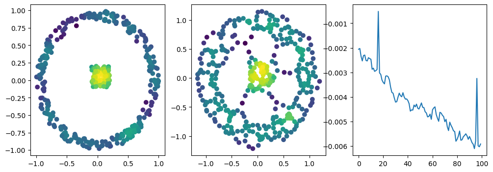
Spatially localized optimization

The goal of this notebook is to generate cycles on the modes of a fixed measure.

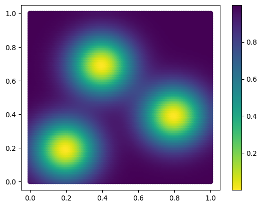
In this example, the measure is defined (in the cell below) as a sum of 3 gaussian measures.

## The density function of the measure
def custom_map(x, sigma=.17, threshold=None):
    if x.ndim == 1:
        x = x[None,:]
    assert x.ndim ==2
    basepoints = t.tensor([[0.2,0.2], [0.8, 0.4], [0.4, 0.7]]).T
    out = -(t.exp( - (((x[:,:,None]- basepoints[None,:,:]) / sigma).square() ).sum(dim=1) )).sum(dim=-1)
    return 1+out # 0.8 pour norme 1

x= np.linspace(0,1,100)
mesh = np.meshgrid(x,x)
coordinates = np.concatenate([stuff.flatten()[:,None] for stuff in mesh], axis=1)
coordinates = torch.from_numpy(coordinates)
plt.scatter(*coordinates.T,c=custom_map(coordinates), cmap="viridis_r")
plt.colorbar()

<matplotlib.colorbar.Colorbar at 0x7f0d9fb51550>

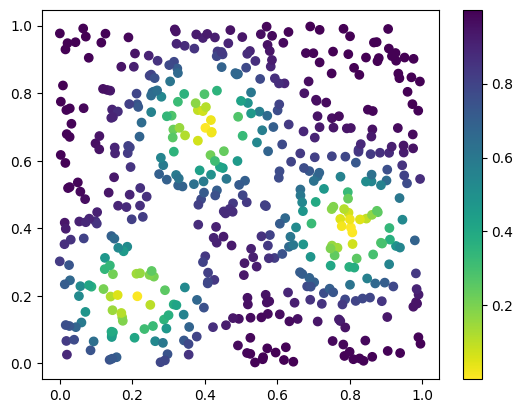
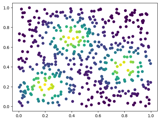
We start from a uniform point cloud, that we will optimize

x = np.random.uniform(size=(500,2))
x = t.tensor(x, requires_grad=True)
plt.scatter(*x.detach().numpy().T, c=custom_map(x).detach().numpy(), cmap="viridis_r")
plt.colorbar()

<matplotlib.colorbar.Colorbar at 0x7f0d9f123f80>

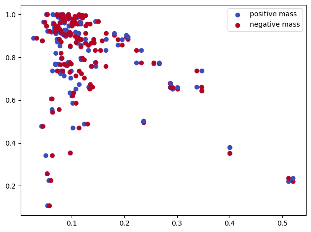
The function_rips_signed_measure function is meant to compute signed measures from rips + function bifiltrations, in a torch-differentiable manner.

x = np.random.uniform(size=(300,2))
x = t.tensor(x, requires_grad=True)
sm_diff, = mpt.function_rips_signed_measure(
    x, function=custom_map, degree=1, num_collapses=-1, plot=True, verbose=True, complex="rips");

For this example we use the following loss. Given a signed measure $\mu$, define

$$\mathrm{loss}(\mu) := \int\varphi(x) d\mu(x)$$

where $x := (r,d)\in \mathbb R^2$ ($r$ for radius, and $d$ for codensity value of the original measure) $$\varphi(x) = \varphi(r,d) = r\times(\mathrm{threshold}-d)$$

This can be interpreted as follows :

• we maximise the radius of the negative point (maximizing the radius of cycles)

• we minimize the radius of positive points (the edges of the connected points creating the cycles). This create pretty cycles

• we care more about cycles that are close to the mode (the threshold-d part). The threshold is meant to prevent the cycles that are not close enough the the cycles to progressively stop to create loops.

threshold = .65
def softplus(x):
    return torch.log(1+torch.exp(x))
# @torch.compile(dynamic=True)
def loss_function(x,sm):
    pts,weights = sm
    radius,density = pts.T
    density = density
    
    phi = lambda x,d : (
        x
        * (threshold-d)
    ).sum()
    loss = phi(radius[weights>0], density[weights>0]) - phi(radius[weights<0], density[weights<0])
    return loss

loss_function(x,sm_diff) #test that it work. It should make no error + have a gradient

tensor(0.2285, grad_fn=<SubBackward0>)

xinit = np.random.uniform(size=(500,2)) # initial dataset
x = t.tensor(xinit, requires_grad=True)
adam = t.optim.Adam([x], lr=0.01) #optimizer
losses = []
plt.scatter(*x.detach().numpy().T, c=custom_map(x, threshold=np.inf).detach().numpy(), cmap="viridis_r")
plt.show()
for i in range(101): # gradient steps
    # change backend to "multipers" if you don't have mpfree
    sm_diff, = mpt.function_rips_signed_measure(x, function=custom_map, degree=1, complex="delaunay"); # delaunay can be changed to rips
    adam.zero_grad()
    loss = loss_function(x,sm_diff)
    loss.backward()
    adam.step()
    losses.append([loss.detach().numpy()])
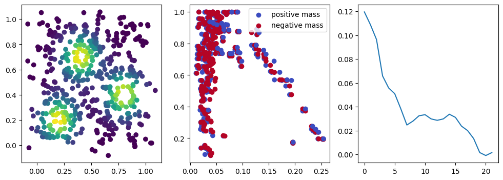
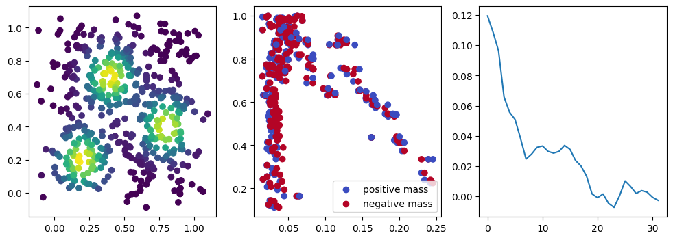
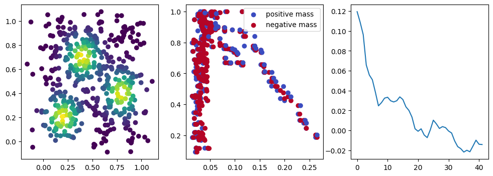
    with torch.no_grad():
        if i %10 == 1: #plot part
            base=4
            ncols=3
            fig, (ax1, ax2, ax3) = plt.subplots(nrows=1, ncols=ncols, figsize=(ncols*base, base))
            ax1.scatter(*x.detach().numpy().T, c=custom_map(x, threshold=np.inf).detach().numpy(), cmap="viridis_r", )
            plot_signed_measure(sm_diff, ax=ax2)
            ax3.plot(losses, label="loss")
            plt.show()
fig, (ax1, ax2, ax3) = plt.subplots(nrows=1, ncols=ncols, figsize=(ncols*base, base))
ax1.scatter(*xinit.T, c=custom_map(t.tensor(xinit)).detach().numpy(),cmap="viridis_r")
ax2.scatter(*x.detach().numpy().T, c=custom_map(x).detach().numpy(),cmap="viridis_r")
ax3.plot(losses)

plt.show()

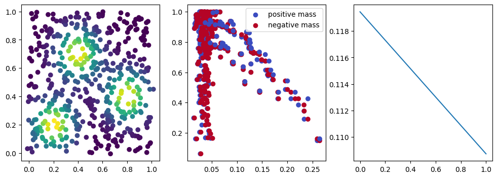
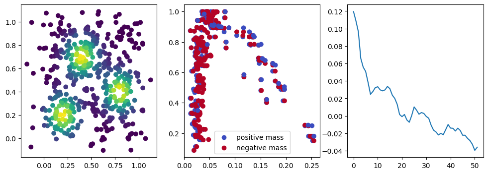
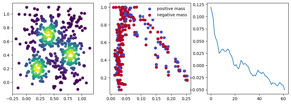
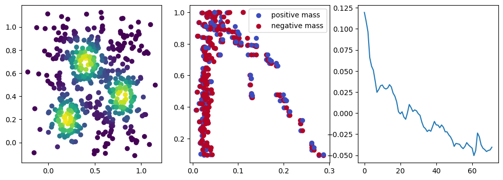
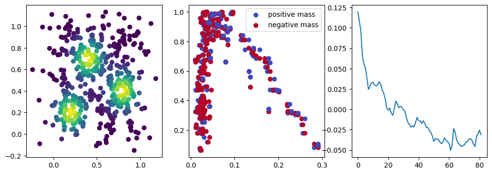
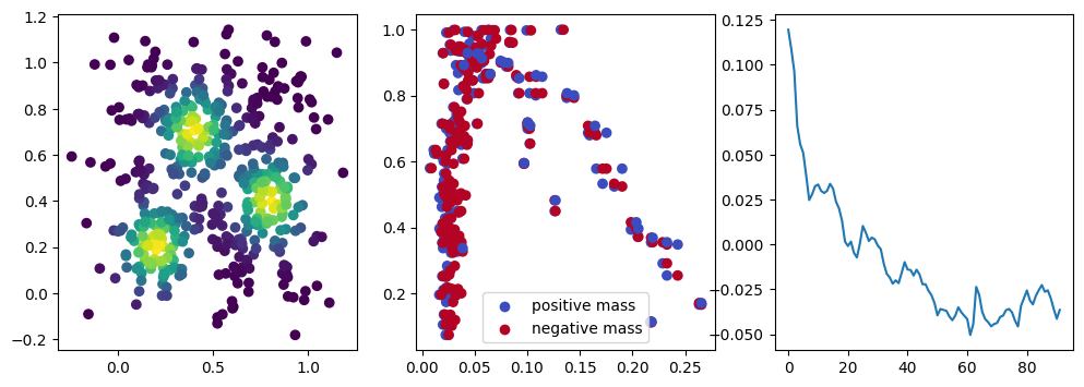
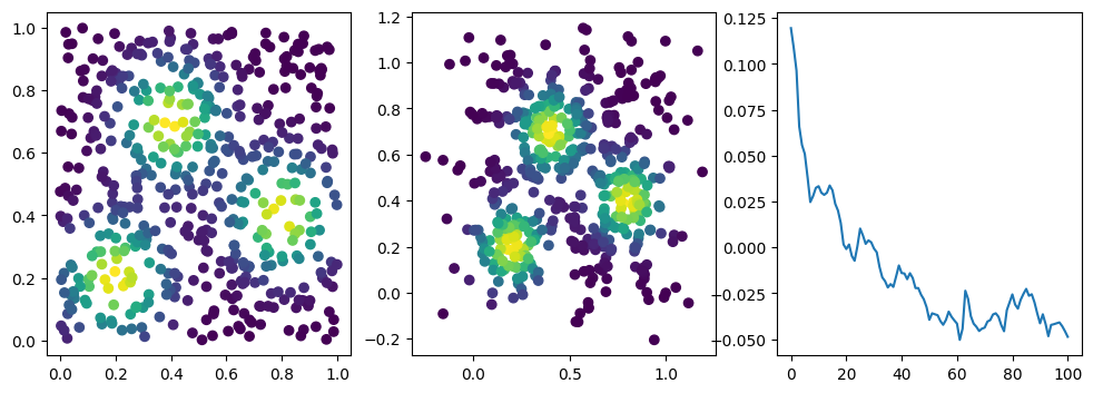
We now observe a onion-like structure around the poles of the background measure.

How to interpret this ? The density constraints (in the loss) and the radius constraints are fighting against each other, therefore, each cycle has to balance itself to a local optimal, which leads to these onion layers.

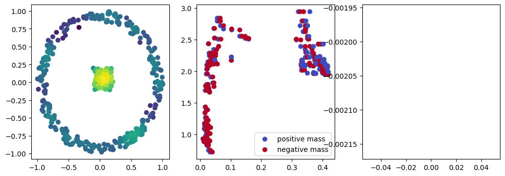
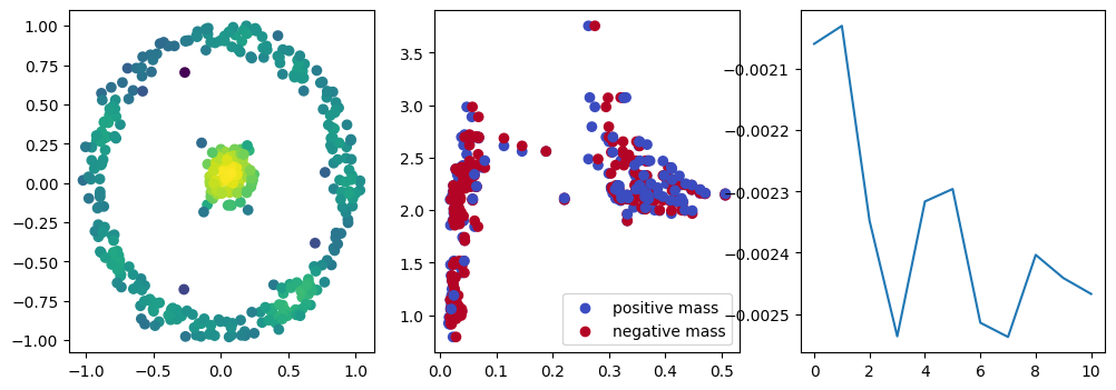
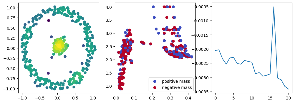
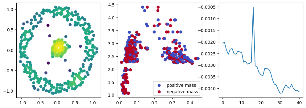
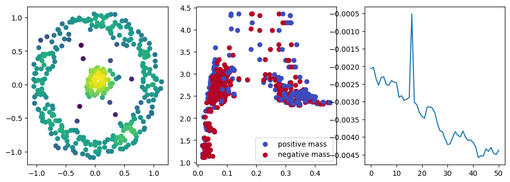
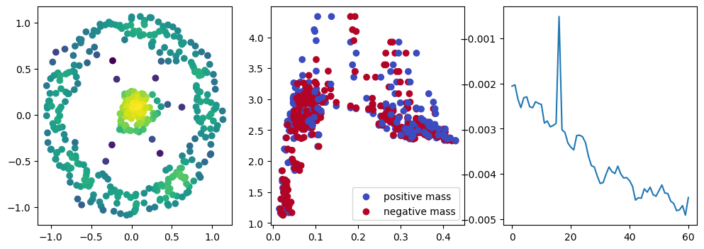
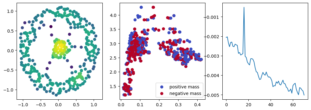
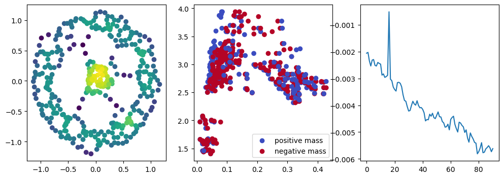
Density preserving optimization

Example taken from the paper Differentiability and Optimization of Multiparameter Persistent Homology, and is an extension of the point cloud experiement of the optimization Gudhi notebook.
One can check from the Gudhi’s notebook that a compacity regularization term is necessary in the one parameter persistence setting; this issue will not happen when optimizing a Rips-Density bi-filtration, as we can enforce cycles to naturally balance between scale and density, and hence not diverge.

from multipers.ml.convolutions import KDE
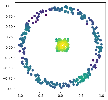
X = np.block([
    [np.random.uniform(low=-0.1,high=.2,size=(100,2))],
    [mp.data.noisy_annulus(300,0, 0.85,1)]
])
bandwidth = .1
custom_map2 = lambda X :  -KDE(bandwidth=bandwidth, return_log=True).fit(X).score_samples(X)
codensity = custom_map2(X)
plt.scatter(*X.T, c=-codensity)
plt.gca().set_aspect(1)

def norm_loss(sm_diff,norm=1.):
    pts,weights = sm_diff
    loss = (torch.norm(pts[weights>0], p=norm, dim=1)).sum() -  (torch.norm(pts[weights<0], p=norm, dim=1)).sum()
    return loss / pts.shape[0]

x = torch.from_numpy(X).clone().requires_grad_(True)
opt = torch.optim.Adam([x], lr=.01)
losses = []
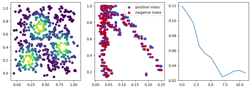
for i in range(100):
    opt.zero_grad()
    sm_diff, = mpt.function_rips_signed_measure(x=x, theta=bandwidth,degrees=[1], kernel="gaussian", complex="delaunay")
    loss = norm_loss(sm_diff)
    loss.backward()
    losses.append(loss)
    opt.step()
    if i % 10 == 0:
    	with torch.no_grad():
            base=4
            ncols=3
            fig, (ax1, ax2, ax3) = plt.subplots(nrows=1, ncols=ncols, figsize=(ncols*base, base))
            ax1.scatter(*x.detach().numpy().T, c=custom_map2(x).detach().numpy(), cmap="viridis_r", )
            plot_signed_measure(sm_diff, ax=ax2)
            ax3.plot(losses, label="loss")
            plt.show()

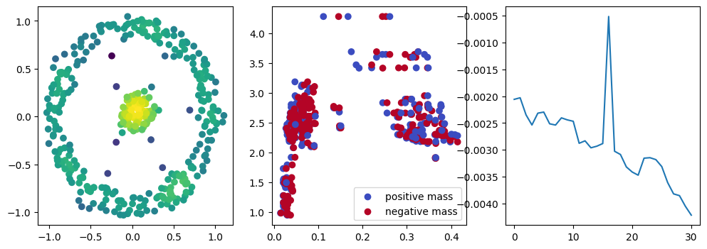
with torch.no_grad():
    fig, (ax1, ax2, ax3) = plt.subplots(nrows=1, ncols=ncols, figsize=(ncols*base, base))
    ax1.scatter(*X.T, c=custom_map2(t.tensor(X)).detach().numpy(),cmap="viridis_r")
    ax2.scatter(*x.detach().numpy().T, c=custom_map2(x).detach().numpy(),cmap="viridis_r")
    ax3.plot(losses)
    plt.show()