Multiparameter persistence introduction

import multipers as mp
import matplotlib.pyplot as plt
import numpy as np
import gudhi as gd
import multipers.point_measure_integration
import multipers.plots as mpp
import multipers.ml.point_clouds as mmp
from multipers.data import noisy_annulus, three_annulus
import multipers.ml.signed_measures as mms
from multipers.ml.convolutions import KDE
np.random.seed(1)

mp.simplex_tree_multi.SAFE_CONVERSION=True ## Enable this if you encounter crashes.

Remark. As we mainly focus on Multiparameter Topological Persistence here, the usual 1-parameter Persistence setting is not well detailed here.
We recommend the reader to familiarize first with persistent homology (on e.g. youtube) to have a better understanding of this notebook.

Point clouds

Topological Persistence and Noise

Let’s start with a standard annulus.

X = noisy_annulus(n1=500, n2=0)
plt.scatter(X[:,0], X[:,1], s=5); plt.gca().set_aspect(1)

As this is very close to the annulus (w.r.t., e.g., the Haussdorff distance), its persistence will be close to the one of the annulus, i.e.,

• In degree 0, one connected component appearing at time 0, and never dying,

• In degree 1, one cycle appearing at time 0, and dying at the diameter of the inner radius of the annulus (1).

More formally, we’re looking at the persistence of topological signal (here homology) along the familly of topological spaces (topological filtration)

$$X = (X_t){t\ge 0} \quad \text{where } X_t := { x \in \mathbb R ^2 : d(x, X) \le t} = \bigcup{x\in X} B(x,t)$$

Now as the topology of $X_t$ change over time ($t$), one can track the appearance of topological signal and its persistence over time.
This is exactly what we recover using Persistent Homology, which gives us, for each such topological signal, its lifetime w.r.t. the time $t$, in a so-called barcode: the familly of bars representing these lifetimes.
Note. These bars can be represented in a Persistence Diagram by coordinates in $\mathbb R^2$ in the coordinate system $(\text{birth}, \text{death})\in \mathbb R^2$.

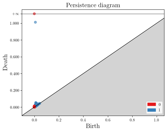
persistence = gd.AlphaComplex(points=X).create_simplex_tree().persistence()
# gd.plot_persistence_barcode(persistence)
gd.plot_persistence_diagram(persistence=persistence)

/home/dloiseau/micromamba/envs/312/lib/python3.12/site-packages/gudhi/persistence_graphical_tools.py:105: UserWarning: This function is not available.
ModuleNotFoundError: No module named 'matplotlib'.
  warnings.warn(f"This function is not available.\nModuleNotFoundError: No module named '{import_error.name}'.")

<Axes: title={'center': 'Persistence diagram'}, xlabel='Birth', ylabel='Death'>

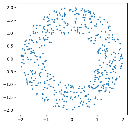
Let’s add some noise now.

X = noisy_annulus(n1=500, n2=500)
plt.scatter(X[:,0], X[:,1], s=5); plt.gca().set_aspect(1)
persistence = gd.AlphaComplex(points=X).create_simplex_tree().persistence()
gd.plot_persistence_diagram(persistence=persistence)

<Axes: title={'center': 'Persistence diagram'}, xlabel='Birth', ylabel='Death'>

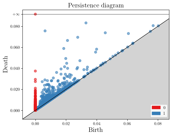
As one can see, the persistence completely changed! and we cannot recover the original annulus, as the few points in the middle filled the gap in the middle.

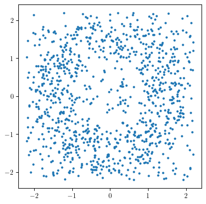
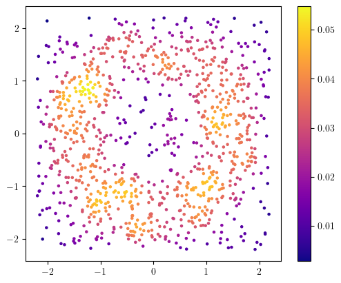
One way to deal with this issue is to take into account the sampling measure of the dataset; it is much more concentrated on the annulus than on the diffuse noise.

density = KDE(bandwidth=0.2).fit(X).score_samples(X)
plt.scatter(X[:,0], X[:,1], s=5, c=(density), cmap="plasma"); plt.gca().set_aspect(1); plt.colorbar();

[KeOps] Warning : Cuda libraries were not detected on the system ; using cpu only mode

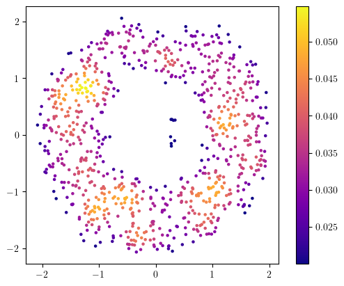
And now, a first idea would be to remove the low density points, which should correspond to some noise

threshold = 0.02
idx = density>threshold
plt.scatter(X[idx,0], X[idx,1], s=5, c=(density[idx]), cmap="plasma"); plt.gca().set_aspect(1), plt.colorbar()

persistence = gd.AlphaComplex(points=X[idx]).create_simplex_tree().persistence()
gd.plot_persistence_diagram(persistence=persistence)

<Axes: title={'center': 'Persistence diagram'}, xlabel='Birth', ylabel='Death'>

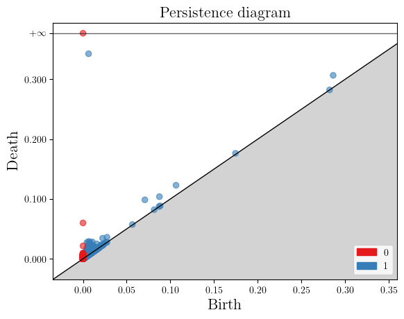
This seems to work! But there are a few caveats, in particular in this (easy) example

• The choice of threshold is easy here, but in practice, this choice is not canonical, and may not even exist,

• The cycle isn’t dying at the proper place (0.4 instead of 1) because of the few points in the middle

A better strategy is to use two parameter persistence. We were using previously the topologial filtration

$$X = (X_t){t\ge 0} \quad \text{where } X_t := { x \in \mathbb R ^2 : d(x, X) \le t} = \bigcup{x\in X} B(x,t)$$

And we’ll add a second axis which will be defined by the codensity of the point cloud. This defines a 2-parameter filtration on which we’ll also track the topological persistence

$$X = (X_{(t,s)}){t\ge 0,s\in \mathbb R} \quad \text{where } X{(t,s)} := { x \in \mathbb R ^2 : d(x, X) \le t, \mathrm{density}(x) \ge s } = \bigcup_{x\in X} B(x,t) \bigcap \mathrm{density}^{-1}(s,\infty)$$

We hide this with the PointCloud2SimplexTree pipeline, but this is detailed in the Custom Multifiltration notebook.

(simplextree,), = mmp.PointCloud2SimplexTree(expand_dim=2,bandwidths=[0.2], num_collapses="full", threshold=2, complex='rips').fit_transform([X])

Multipersistence representations

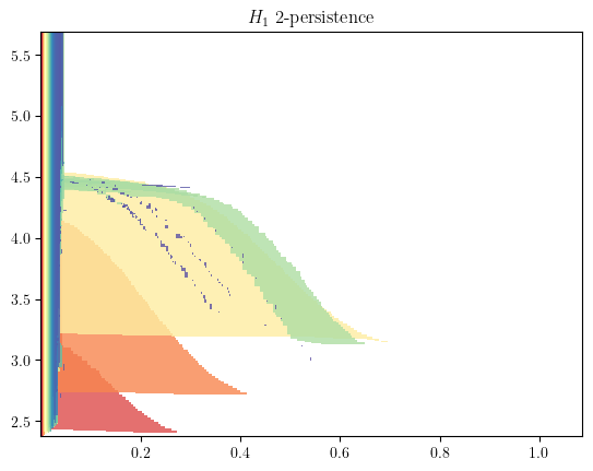
Multiparameter Module Approximation (MMA)

Note: In this subsection, we focus on “multipers-only” functions; a bunch of steps can be significantly speed up using external libraries, as showcased in next sections.

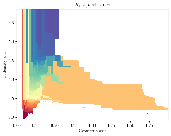
A representation of the 2 persistence can be computed using interval decomposition technics, such as our multiparameter_module_approximation module. Theoretical definitions can be found in the MMA paper.
Here each interval, i.e., colored shape, visually correspond to the lifetime of a cycle in this 2-filtration.
You can morally interpret this as a barcode for each density horizontal stratum that are properly glued vertically together.
As you can see, there is one significant shape that stands out, which correspond to the annulus.

bimod = mp.module_approximation(simplextree)
bimod.plot(degree=1)
plt.xlabel('Geometric axis')
plt.ylabel('Codensity axis')

Text(0, 0.5, 'Codensity axis')

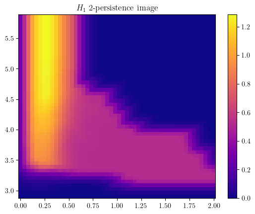
Surprisingly, these approximations can be used to compute very efficiently Multiparameter Persistent Landscapes, or any vectorization from A Framework for MPH Decompositions Representations. This makes MMA modules a very good structure to compute for hyperparameter cross validation!

bimod.landscapes(degree=1, ks=range(5), plot=True); # Landscape of degree one with k=0,1,2,3,4

bimod.representation(degrees=[1], bandwidth=-.1, plot=True, p=2, kernel="linear"); # An image representation of the bimod

The multipers.ml.mma module, containing (among other) MMAFormatter, MMA2Img, MMA2Landscape can also help you to achieve this in a more scalable way

Signed Barcode Decompositions as Signed Measures

Although this structure is more visually intepretable, it can still be too expensive to compute depending on the usecase.
An alternative option, is to compute Signed Barcode, which provide a bunch of weaker topological invariants, that can be used in a ML context as Signed Measures.
This library has several of them :

• Hilbert function decomposition,

• Rank decomposition (via rectangles),

• Euler Characteristic decomposition.

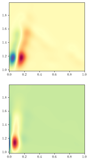
The easiest to understand might be the hilbert signed measure, which is derived from the dimension vector of this previous 2-parameter module.
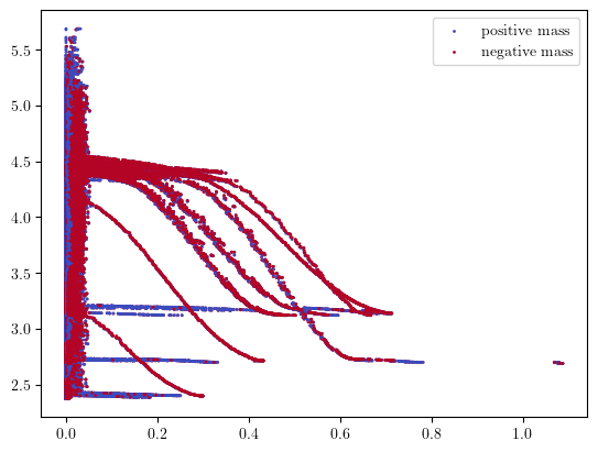
In the figure below, on the left you have the pointwise dimension of the bimodule (a.k.a. The Hilbert Function), and on the right its associated signed measure, that can be interpreted as the “changes” of values of the hilbert function on the left.

fig, (ax1, ax2) = plt.subplots(ncols=2, nrows=1, figsize=(10,4))
hilbert_sm = mp.signed_measure(simplextree, degree=1)
surface, grid =  mp.point_measure_integration.integrate_measure(*hilbert_sm[0], return_grid=True)
mpp.plot_surface(grid, surface, discrete_surface=True, ax=ax1)
mpp.plot_signed_measure(*hilbert_sm, ax=ax2)

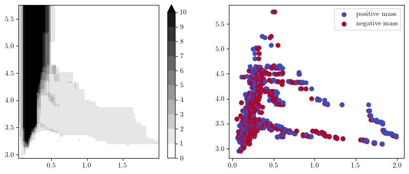
You can interpret the measure on the right as follows

• each blue dot correspond to “something that appear in homology at this grade”

• each red dot correspond to “something that dies in homology at this grade”

We refer the reader to the Signed Measures paper for formal definitions.

Signed measures can also be computed from different topological invariant derived from a $n$-parameter persistence module, e.g., the Euler characteristic, which leads to the Euler signed masure. This one can be very fast to compute, but is not well suited to be used on point clouds, as it has to be computed on the full simplicial complex, i.e., using the simplices of all dimension, which can be prohibitive to store.
In this example, we compute this invariant on a regular smaller subgrid to be able to hold this invariant in memory.

simplextree.expansion(simplextree.num_vertices)
euler_sm = mp.signed_measure(simplextree, degree=None, plot=True);

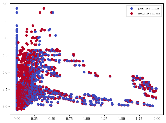
Or the rank invariant decompositions, which is in general harder to compute than MMA modules, but can be restricted to smaller subgrids to have reasonable compute times.

simplextree.prune_above_dimension(2) ## The simplices above dimension 2 are not necessary here; this speeds up the computations.
rank_sm = mp.signed_measure(simplextree,degree=1, invariant = "rank", plot = True, grid_strategy = "regular", resolution=50);

These measures can also easily be turned into vectors using the SignedMeasure2Convolution method

[hilbert_sm, euler_sm] = mms.SignedMeasureFormatter(normalize=True).fit_transform([hilbert_sm, euler_sm]) ## for better plots, we normalize the filtrations
mms.SignedMeasure2Convolution(plot=True, bandwidth=.05, grid_strategy="regular", resolution=200).fit_transform([hilbert_sm, euler_sm]);

[KeOps] Generating code for formula Sum_Reduction((Exp(-Sum(((Var(0,2,0)-Var(1,2,1))/Var(2,1,2))**2)/2)/Var(3,1,2))*Var(4,1,0),1) ... OK
[pyKeOps] Compiling pykeops cpp 529fbbcb99 module ... OK

Another approach, with external libraries

We consider the same strategy as above but with another dataset. We will see that we are able to use the concentration of the sampling measure to our adventage.
Rips can become quite large on bigger datasets, so we will consider Function Delaunay bifiltrations instead, on which we compute minimal presentation to compute our invariants, with mpfree.

You will need these two dependencies to execute the following code. FunctionDelaunay and mpfree.

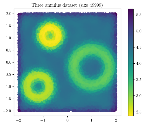
X = three_annulus(25_000,25_000)
density = KDE(bandwidth=0.15, return_log=True).fit(X).score_samples(X)
plt.scatter(*X.T, c = -density, cmap="viridis_r")
plt.gca().set_aspect(1); plt.colorbar()

<matplotlib.colorbar.Colorbar at 0x7fb52a913ec0>

We first compute the Density-Delaunay bifiltration using

import multipers.slicer as mps
function_delaunay = mps.from_function_delaunay(X,-density) ## needs function_delaunay

On which we compute the minimal presentation of degree 1, using mpfree.

minimal_presentation = mps.minimal_presentation(function_delaunay, degree = 1) ## needs mpfree
# Note. These two steps can be done faster by providing the degree to function_delaunay

There are different options there, but in this case we end up with a Slicer structure, which can be used to compute our previous invariant, in a much quicker way.

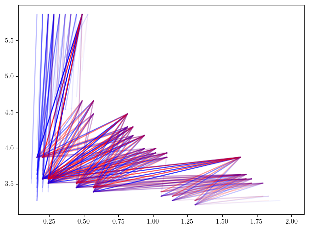
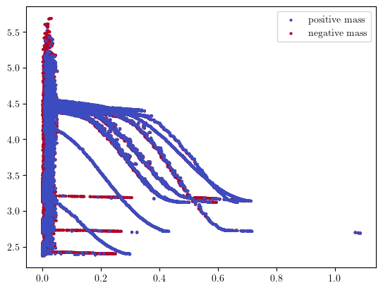
As expected, we can clearly distinguish the 3 circles as the 3 big shapes in the figure below, and identify them using their radii. The surprising part is that multiparameter persistence also allows us to identify them using the concentration of their sampling ! This allows to retrieve much more information from the dataset :)
Exercice: Can you identify where is the 4th cycle in the original dataset ?

mp.module_approximation(minimal_presentation, direction=[1,0], swap_box_coords=[1]).plot(1, alpha=.8)
# Note. The optinal parameters are meant to speed up computations in this specific context, and can be removed. Plot also takes a lot of time here

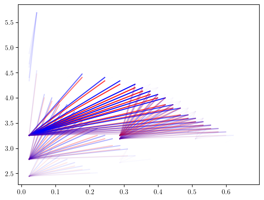
The Hilbert Signed measure can be directly retrieved from the minimal resolution, as the euler charteristic of the minimal free resolution is the hilbert function.

hilbert_sm, = mp.signed_measure(minimal_presentation)
mpp.plot_signed_measure(hilbert_sm, s=4)

rank_sm, = mp.signed_measure(mp.Slicer(minimal_presentation, vineyard=False, dtype=minimal_presentation.dtype), invariant = "rank", degree=1, grid_strategy = "regular_closest", resolution=50)
mpp.plot_signed_measure(rank_sm, s=4)

The euler characteristic can be computed from the original function delaunay (with all of the simplices)

euler_sm, = mp.signed_measure(function_delaunay, clean=True) ## Clean create smaller measures for euler
mpp.plot_signed_measure(euler_sm, s=1)