Improving the evaluation using the Jacobian and centered form

Let $x_j^m$ be the middle point of $(\underline{x_j},\overline{x_j})$ and $X=\{(\underline{x_1},\overline{x_1}),\ldots,(\underline{x_m},\overline{x_m})\}$ be the box. Then:

$$(\underline{F_j(X)},\overline{F_j(X)}) \in F_j(x_1^m,\ldots,... ...ldots,(\underline{x_i},\overline{x_i}),x_{i+1}^m,\ldots,x_m^m)$$ (2.4)

see [5], pp. 52. This expression enable to get in some cases a sharper bound on $F_j$.

This evaluation is embedded into the evaluation procedure of the solving algorithms using the Jacobian. It is also available in its general form as

 
INTERVAL_VECTOR Centered_Form(int DimVar,int DimEq,
          INTERVAL_VECTOR (* TheIntervalFunction)(int,int,INTERVAL_VECTOR &), 
          INTERVAL_MATRIX (* Gradient)(int, int, INTERVAL_VECTOR &), 
          VECTOR &Center,
          INTERVAL_VECTOR &Input)

where

• DimVar: number of variables
• DimEq: number of expressions
• TheIntervalFunction: procedure in MakeF format for interval evaluating the expressions
• Gradient: procedure un MakeJ format for evaluating the derivatives of the expressions
• Center:the center point for the centered form
• Input: the ranges for the variables

A variant of this procedure is

 
INTERVAL Centered_Form(int k,int DimVar,int DimEq,
          INTERVAL_VECTOR (* TheIntervalFunction)(int,int,INTERVAL_VECTOR &), 
          INTERVAL_MATRIX (* Gradient)(int, int, INTERVAL_VECTOR &), 
          VECTOR &Center,
          INTERVAL_VECTOR &Input)

which is used to evaluate only expression number $k$.

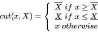
A more sophisticated evaluation for the centered form is based on Baumann theorem [18]. First we define the procedure cut(double x,INTERVAL X) as:

$$cut(x,X)=\left\{ \begin{array}{c} \overline{X}~if~x\ge \ov... ...{X}~if~x\le \underline{X}\\ x~otherwise \end{array} \right.$$

For a system of $m$ equations $F$ in $n$ unknowns $X$ we define

$$p^l_k = cut(\frac{Mid((\partial F^\prime_l/\partial X_k)(X))}{Diam((\partial F^\prime_l/\partial X_k)(X))},[-1,1])$$

For a given equation $l$ we use the centered form with as center

$$x^1_k=Mid(X_k)-p^l_kDiam(X_k)~~~x^2_k=Mid(X_k)-p^l_kDiam(X_k)$$

with $k$ in $[1,n]$. The choice for $x^1, x^2$ is based on the property that the lower end-point of the centered form $F(x,X)$ has a maximum at $x^2$ while its upper end-point has a minimum at $x^1$. The interval evaluation of $F_l$ is obtained as $F_l(x^1,X) \cap F_l(x^2,X)$. Although $2nm$ centered form are used to compute the interval evaluation of the $m$ equations the calculation is in fact not so expensive as the interval evaluation of the Jacobian matrix has to be done only once.

The implementation is:

 
INTERVAL_VECTOR BiCentered_Form(int DimVar,
          int DimEq,
          INTERVAL_VECTOR (* TheIntervalFunction)(int,int,INTERVAL_VECTOR &), 
          INTERVAL_MATRIX (* Gradient)(int, int, INTERVAL_VECTOR &), 
          INTERVAL_VECTOR &Input,
          int Exact)

where

• DimVar: number of variables
• DimEq: number of expressions
• TheIntervalFunction: procedure in MakeF format for interval evaluating the expressions
• Gradient: procedure un MakeJ format for evaluating the derivatives of the expressions
• Input: the ranges for the variables
• Exact: if 0 the procedure will return as soon as an interval evaluation of one expression does not include 0

A variant for evaluating only equation number $k$ is

 
INTERVAL_VECTOR BiCentered_Form(int k,int DimVar,
          int DimEq,
          INTERVAL_VECTOR (* TheIntervalFunction)(int,int,INTERVAL_VECTOR &), 
          INTERVAL_MATRIX (* Gradient)(int, int, INTERVAL_VECTOR &), 
          INTERVAL_VECTOR &Input,
          int Exact)

Another variant is based on the property that the numerical interval evaluation of the product J(Input)(Input-Center) may be overestimated as there may be several occurence of the same variable in this product. We may assume that this product has been computed symbolically, then re-arranged to reduce the number of occurence of the same variable leading to a procedure in MakeF format that computes directly the product. The syntax of the bicentered form procedure is

 
INTERVAL_VECTOR BiCentered_Form(int DimVar,
          int DimEq,
          INTERVAL_VECTOR (* TheIntervalFunction)(int,int,INTERVAL_VECTOR &), 
          INTERVAL_MATRIX (* Gradient)(int, int, INTERVAL_VECTOR &), 
          INTERVAL_VECTOR (* ProdGradient)(int, int, INTERVAL_VECTOR &), 
          INTERVAL_VECTOR &Input,
          int Exact)

where ProdGradient is the procedure that computes the product J(Input)(Input-Center), being understood that the Center is available in the global variable ALIAS_Center_CenteredForm.