Estimation of the model parameters

In case the observed texture was found to contain harmonic components, we employ an iterative procedure to estimate the texture parameters. In each iteration the frequency of the dominant harmonic component is estimated by :

$$(\hat \omega_p, \hat \nu_p) = \mathop{\rm arg max}\limits_{(\... ...\nu)} \bigg \vert {\rm DFT}\bigg (y(n,m)\bigg ) \bigg\vert \ .$$

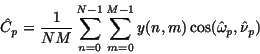
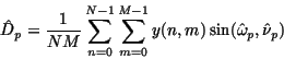
Then, we may use a demodulation procedure to estimate the amplitudes of the harmonic components :

$$\hat C_p = \frac{1}{NM} \sum_{n=0}^{N-1} \sum_{m=0}^{M-1}y(n,m)\cos(\hat \omega_p, \hat \nu_p)$$

and similarly :

$$\hat D_p = \frac{1}{NM} \sum_{n=0}^{N-1} \sum_{m=0}^{M-1}y(n,m)\sin(\hat \omega_p, \hat \nu_p)$$

where the dimensions of the observed image are $N\times M$. Next we subtract the estimated harmonic component from the observed signal y(n,m) and repeat this procedure iteratively until all harmonic components whose magnitude is higher than the foregoing test threshold are extracted. The residual field is the purely-indeterministic component of the texture.

The frequency parameter $\nu_{i}^(\alpha,\beta)$ and the $(\alpha_{i},\beta_{i})$can be easily estimated using standard techniques (Hough transform).

A procedure of demodulation of the evanescent component provides estimates of the 1-D sequences $\{ s_i^{(\alpha ,\beta)}(n \alpha -m \beta) \}$ and $\{ t_i^{(\alpha ,\beta)}(n \alpha -m \beta) \}$ of each evanescent field. Finally, these sequences are fitted with their 1-D AR models. The removal of all evanescent components of the field leaves us with a residual field which is the purely-indeterministic component of the texture.

The parameters of the purely-indeterministic component are estimated using a computationally efficient algorithm for estimating its moving average model. The algorithm first fits a 2-D NSHP AR model to the observed field, by using a ML algorithm. Note that in this case, where all the deterministic components have already been removed, the procedure of obtaining a maximum-likelihood estimate of the AR model parameters is reduced to a solution of a linear least squares problem. In the second stage, the estimated parameters of the AR model are employed to compute the parameters of the moving average model, through a least squares solution of a system of linear equations.