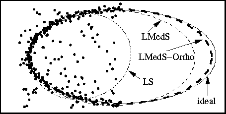
Figure 9: Comparison of different techniques in the presence of outliers in data
We now introduce outliers in the above set of noisy data points. The outliers are generated by a uniform distributed noise in an rectangle whose lower left corner is at (140, 195) and whose upper right corner is at (250, 305). The complete set of data points are shown as black dots in fig:res-outliers.

Figure 9: Comparison of different techniques in the presence of outliers in
data
In fig:res-outliers, we show the ellipse estimated by the linear least-squares without outliers rejection (shown in dotted lines) which is definitely very bad, the ellipse estimated by the least-median-squares without continued by the weighted least-squares (LMedS) (shown in thin dashed lines) which is quite reasonable, and the ellipse estimated by the least-median-squares continued by the weighted least-squares (LMedS-complete) (shown in thick dashed lines) which is very close to the ideal ellipse. The ellipse parameters estimated by these techniques are compared in Table 4.

Table 4: Comparison of the estimated parameters by non-robust and robust techniques
The computation time on a Sun Sparc 20 workstation is respectively 0.008 seconds, 2.56 seconds, and 6.93 seconds for linear least-square, LMedS and LMedS-complete. Please bear in mind that the time given here is only for illustration since I did not try to do any code optimization. The most time-consuming part is the computation of the orthogonal distance between each point and the ellipse.