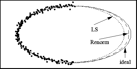
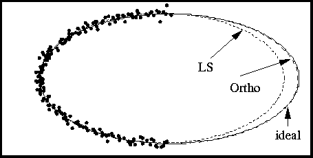
The ideal ellipse used in our experiment has the following parameters: the long
axis is equal to 100 pixels, the short axis is equal to 50 pixels, the center
is at (250, 250), and the angle between the long axis and the horizontal
axis is 0 ![]() . The left half section of the ellipse is used and is
sampled by 181 points. Finally, a Gaussian noise with 2 pixels of standard
deviation is added to each sample points, as shown by black dots in
fig:res-LS-RENORM and fig:res-LS-ORTHO, where the ideal ellipse is
also shown in solid lines.
. The left half section of the ellipse is used and is
sampled by 181 points. Finally, a Gaussian noise with 2 pixels of standard
deviation is added to each sample points, as shown by black dots in
fig:res-LS-RENORM and fig:res-LS-ORTHO, where the ideal ellipse is
also shown in solid lines.
The linear least-squares technique, the renormalization technique, and the technique based on orthogonal distances between points and ellipse are applied to the noisy data. A visual comparison of the results is shown in fig:res-LS-RENORM and fig:res-LS-ORTHO. A quantitative comparison of the estimated parameters is described in Table 2. As can be observed, the linear technique introduces a significant bias (this is more prominent if a shorter section of ellipse is used). The renormalization technique corrects the bias and improves considerably the result (however, because of the underlying statistical assumption, this technique does not work as well if only a small set of data is available). The technique based on the minimization of orthogonal distances definitely gives the best result.

Figure 7: Comparison between Linear Least-Squares (LS, in dotted
lines) and Renormalization technique (Renorm, in dashed lines)

Figure 8: Comparison between Linear Least-Squares (LS) and Orthogonal Regression (Ortho)

Table 2: Comparison of the estimated parameters by different techniques
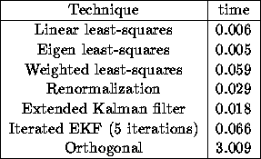
Table 3 shows roughly the computation time required for each method. Eigen least-squares yields similar result to that of Linear least-squares. Weighted least-squares improves the result a little bit, but not as much as Renormalization for this set of data. Extended Kalman filter or Iterated EKF requires a quite good initial estimate.

Table 3: Comparison of computation time of different techniques:
real time on a SUN Sparc 20 workstation (in seconds)