The least-median-of-squares (LMedS) method estimates the parameters by solving the nonlinear minimization problem:
![]()
That is, the estimator must yield the smallest value for the median of squared residuals computed for the entire data set. It turns out that this method is very robust to false matches as well as outliers due to bad localization. Unlike the M-estimators, however, the LMedS problem cannot be reduced to a weighted least-squares problem. It is probably impossible to write down a straightforward formula for the LMedS estimator. It must be solved by a search in the space of possible estimates generated from the data. Since this space is too large, only a randomly chosen subset of data can be analyzed. The algorithm which we describe below for robustly estimating a conic follows that structured in [22, Chap.,], as outlined below.
Given n points: ![]() .
.
![]()
Here, we have a number of choices for ![]() , the residual
of the ipoint with respect to the conic
, the residual
of the ipoint with respect to the conic ![]() . Depending on the
demanding precision, computation requirement, etc., one can use the
algebraic distance, the Euclidean distance, or the gradient weighted distance.
. Depending on the
demanding precision, computation requirement, etc., one can use the
algebraic distance, the Euclidean distance, or the gradient weighted distance.
By requiring that P must be near 1, one can determine m for given values
of p and ![]() :
:
![]()
In our implementation, we assume ![]() and require
P=0.99, thus m=57. Note that the algorithm can be speeded up considerably
by means of parallel computing, because the processing for each subsample can
be done independently.
and require
P=0.99, thus m=57. Note that the algorithm can be speeded up considerably
by means of parallel computing, because the processing for each subsample can
be done independently.
As noted in [22], the LMedS efficiency is poor in the presence of Gaussian noise. The efficiency of a method is defined as the ratio between the lowest achievable variance for the estimated parameters and the actual variance provided by the given method. To compensate for this deficiency, we further carry out a weighted least-squares procedure. The robust standard deviation estimate is given by
![]()
where ![]() is the minimal median. The constant 1.4826 is a
coefficient to achieve the same efficiency as a least-squares in the
presence of only Gaussian noise; 5/(n-p) is to compensate the effect
of a small set of data. The reader is referred to [22, page
202,]
for the details of these magic numbers. Based on
is the minimal median. The constant 1.4826 is a
coefficient to achieve the same efficiency as a least-squares in the
presence of only Gaussian noise; 5/(n-p) is to compensate the effect
of a small set of data. The reader is referred to [22, page
202,]
for the details of these magic numbers. Based on ![]() , we can assign
a weight for each correspondence:
, we can assign
a weight for each correspondence:

where ![]() is the residual of the ipoint with respect to the conic
is the residual of the ipoint with respect to the conic ![]() .
The correspondences having
.
The correspondences having ![]() are outliers and should not be further
taken into account. The conic
are outliers and should not be further
taken into account. The conic ![]() is finally estimated by
solving the weighted least-squares problem:
is finally estimated by
solving the weighted least-squares problem:
![]()
using one of the numerous techniques described before. We have thus robustly estimated the conic because outliers have been detected and discarded by the LMedS method.
As said previously, computational efficiency of the LMedS method can be
achieved by applying a Monte-Carlo type technique. However, the five points
of a subsample thus generated may be very close to each other. Such a
situation should be avoided because the estimation of the conic
from such points is highly instable and the result is useless. It is a waste
of time to evaluate such a subsample. In order to achieve higher stability and
efficiency, we develop a regularly random selection method based on
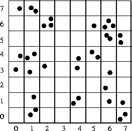
bucketing techniques, which works as follows. We first calculate the min
and max of the coordinates of the points in the first image. The region
is then evenly divided into ![]() buckets (see
fig:bucketing; in our implementation, b=8). To
each bucket is attached a set of points, and indirectly a set of matches,
which fall in it. The buckets having no matches attached are excluded. To
generate a subsample of 5 points, we first randomly select 5 mutually
different buckets, and then randomly choose one match in each selected bucket.
buckets (see
fig:bucketing; in our implementation, b=8). To
each bucket is attached a set of points, and indirectly a set of matches,
which fall in it. The buckets having no matches attached are excluded. To
generate a subsample of 5 points, we first randomly select 5 mutually
different buckets, and then randomly choose one match in each selected bucket.

Figure 5: Illustration of a bucketing technique
One question remains: How many subsamples are required? If we assume that bad
points are uniformly distributed in space, and if each bucket has
the same number of points and the random selection is uniform, the formula
(33) still holds. However, the number of points in one bucket
may be quite different from that in another. As a result, a point belonging to
a bucket having fewer points has a higher probability to be selected. It is
thus preferred that a bucket having many points has a higher probability to
be selected than a bucket having few points, in order that each point has
almost the same probability to be selected. This can be realized by the
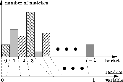
following procedure. If we have in total l buckets, we divide ![]() into
l intervals such that the width of the
into
l intervals such that the width of the ![]() interval is equal to
interval is equal to
![]() , where
, where ![]() is the number of points attached to the
is the number of points attached to the
![]() bucket (see fig:prob-mapping). During the bucket
selection procedure, a number, produced by a
bucket (see fig:prob-mapping). During the bucket
selection procedure, a number, produced by a ![]() uniform random
generator, falling in the
uniform random
generator, falling in the ![]() interval implies that the
interval implies that the
![]() bucket is selected.
bucket is selected.

Figure 6: Interval and bucket mapping
We have applied this technique to matching between two uncalibrated images [24]. Given two uncalibrated images, the only available geometric constraint is the epipolar constraint. The idea underlying our approach is to use classical techniques (correlation and relaxation methods in our particular implementation) to find an initial set of matches, and then use the Least Median of Squares (LMedS) to discard false matches in this set. The epipolar geometry can then be accurately estimated using a meaningful image criterion. More matches are eventually found, as in stereo matching, by using the recovered epipolar geometry.