M-estimators

One popular robust technique is the so-called M-estimators. Let be the residual of the datum, the difference between the observation and its fitted value. The standard least-squares method tries to minimize , which is unstable if there are outliers present in the data. Outlying data give an effect so strong in the minimization that the parameters thus estimated are distorted. The M-estimators try to reduce the effect of outliers by replacing the squared residuals by another function of the residuals, yielding

where is a symmetric, positive-definite function with a unique minimum at zero, and is chosen to be less increasing than square. Instead of solving directly this problem, we can implement it as an iterated reweighted least-squares one. Now let us see how.

Let be the parameter vector to be estimated. The M-estimator of based on the function is the vector which is the solution of the following m equations:

where the derivative is called the influence function. If now we define a weight function

then Equation (29) becomes

This is exactly the system of equations that we obtain if we solve the following iterated reweighted least-squares problem

where the superscript indicates the iteration number. The weight should be recomputed after each iteration in order to be used in the next iteration.

The influence function measures the influence of a datum on the value of the parameter estimate. For example, for the least-squares with , the influence function is , that is, the influence of a datum on the estimate increases linearly with the size of its error, which confirms the non-robusteness of the least-squares estimate. When an estimator is robust, it may be inferred that the influence of any single observation (datum) is insufficient to yield any significant offset [18]. There are several constraints that a robust M-estimator should meet:

• The first is of course to have a bounded influence function.
• The second is naturally the requirement of the robust estimator to be unique. This implies that the objective function of parameter vector to be minimized should have a unique minimum. This requires that the individual -function is convex in variable . This is necessary because only requiring a -function to have a unique minimum is not sufficient. This is the case with maxima when considering mixture distribution; the sum of unimodal probability distributions is very often multi-modal. The convexity constraint is equivalent to imposing that is non-negative definite.
• The third one is a practical requirement. Whenever is singular, the objective should have a gradient, . This avoids having to search through the complete parameter space.

  
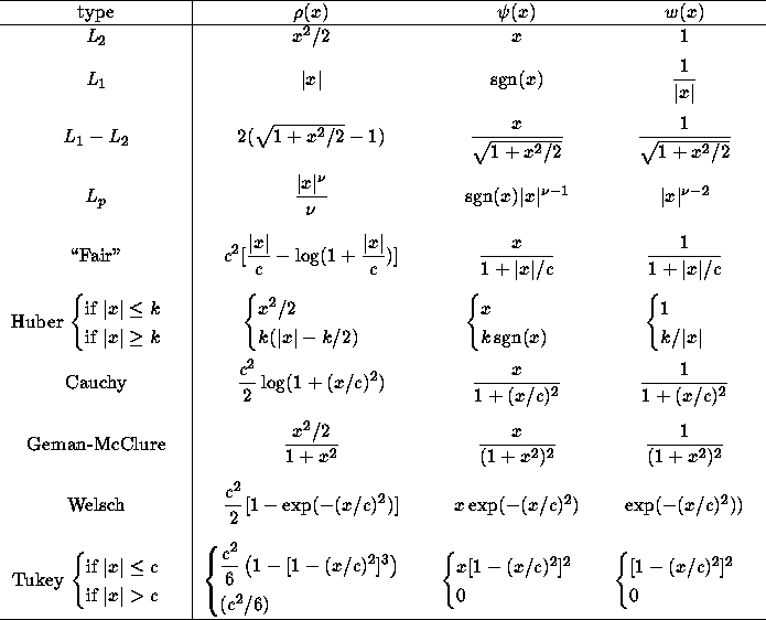
Table 1: A few commonly used M-estimators

  
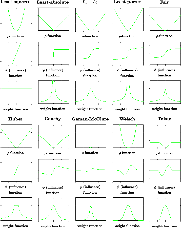
Figure 4: Graphic representations of a few common M-estimators

Briefly we give a few indications of these functions:

• (least-squares) estimators are not robust because their influence function is not bounded.
• (absolute value) estimators are not stable because the -function |x| is not strictly convex in x. Indeed, the second derivative at x=0 is unbounded, and an indeterminant solution may result.
• estimators reduce the influence of large errors, but they still have an influence because the influence function has no cut off point.
• estimators take both the advantage of the estimators to reduce the influence of large errors and that of estimators to be convex.
• The (least-powers) function represents a family of functions. It is with and with . The smaller , the smaller is the incidence of large errors in the estimate . It appears that must be fairly moderate to provide a relatively robust estimator or, in other words, to provide an estimator scarcely perturbed by outlying data. The selection of an optimal has been investigated, and for around 1.2, a good estimate may be expected [18]. However, many difficulties are encountered in the computation when parameter is in the range of interest , because zero residuals are troublesome.
• The function ``Fair'' is among the possibilities offered by the Roepack package (see [18]). It has everywhere defined continuous derivatives of first three orders, and yields a unique solution. The 95% asymptotic efficiency on the standard normal distribution is obtained with the tuning constant c=1.3998.
• Huber's function [7] is a parabola in the vicinity of zero, and increases linearly at a given level |x| > k. The 95% asymptotic efficiency on the standard normal distribution is obtained with the tuning constant k = 1.345. This estimator is so satisfactory that it has been recommended for almost all situations; very rarely it has been found to be inferior to some other -function. However, from time to time, difficulties are encountered, which may be due to the lack of stability in the gradient values of the -function because of its discontinuous second derivative:

  

  The modification proposed in [18] is the following

  The 95% asymptotic efficiency on the standard normal distribution is obtained with the tuning constant c=1.2107.

• Cauchy's function, also known as the Lorentzian function, does not guarantee a unique solution. With a descending first derivative, such a function has a tendency to yield erroneous solutions in a way which cannot be observed. The 95% asymptotic efficiency on the standard normal distribution is obtained with the tuning constant c=2.3849.
• The other remaining functions have the same problem as the Cauchy function. As can be seen from the influence function, the influence of large errors only decreases linearly with their size. The Geman-McClure and Welsh functions try to further reduce the effect of large errors, and the Tukey's biweight function even suppress the outliers. The 95% asymptotic efficiency on the standard normal distribution of the Tukey's biweight function is obtained with the tuning constant c=4.6851; that of the Welsch function, with c=2.9846.

There still exist many other -functions, such as Andrew's cosine wave function. Another commonly used function is the following tri-weight one:

where is some estimated standard deviation of errors.

It seems difficult to select a -function for general use without being rather arbitrary. Following Rey [18], for the location (or regression) problems, the best choice is the in spite of its theoretical non-robustness: they are quasi-robust. However, it suffers from its computational difficulties. The second best function is ``Fair'', which can yield nicely converging computational procedures. Eventually comes the Huber's function (either original or modified form). All these functions do not eliminate completely the influence of large gross errors.

The four last functions do not guarantee unicity, but reduce considerably, or even eliminate completely, the influence of large gross errors. As proposed by Huber [7], one can start the iteration process with a convex -function, iterate until convergence, and then apply a few iterations with one of those non-convex functions to eliminate the effect of large errors.