Consider the biquadratic representation of an ellipse:
![]()
Given n noisy points ![]() (
( ![]() ), we want to
estimate the coefficients of the ellipse:
), we want to
estimate the coefficients of the ellipse: ![]() .
Due to the homogeneity, we set
.
Due to the homogeneity, we set ![]() .
.
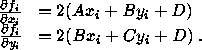
For each point ![]() , we thus have one scalar equation:
, we thus have one scalar equation:
![]()
where
![]()
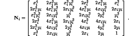
Hence, ![]() can be estimated by minimizing the following objective
function (weighted least-squares optimization)
can be estimated by minimizing the following objective
function (weighted least-squares optimization)
where ![]() 's are positive weights.
's are positive weights.
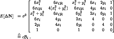
Assume that each point has the same error distribution with mean zero and
covariance 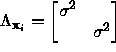 . The covariance of
 ![]() is then given by
is then given by
![]()
where
Thus we have
![]()
The weights can then be chosen to the inverse proportion of the variances. Since multiplication by a constant does not affect the result of the estimation, we set
![]()
The objective function (16) can be rewritten as
![]()
which is a quadratic form in unit vector ![]() . Let
. Let
![]()
The solution is the
eigenvector of ![]() associated to the smallest eigenvalue.
associated to the smallest eigenvalue.
If each point ![]() is perturbed by noise of
is perturbed by noise of ![]() with
with
![]()
the matrix ![]() is perturbed accordingly:
is perturbed accordingly: ![]() , where
, where ![]() is the unperturbed matrix.
If
is the unperturbed matrix.
If ![]() , then the estimate is statistically unbiased; otherwise,
it is statistically biased, because following the perturbation theorem
the bias of
, then the estimate is statistically unbiased; otherwise,
it is statistically biased, because following the perturbation theorem
the bias of ![]() , i.e.,
, i.e., ![]() .
.
Let ![]() , then
, then ![]() . We have
. We have
If we carry out the Taylor development and ignore quantities of order higher
than 2, it can be shown that the expectation of ![]() is given by
is given by
It is clear that if we define
![]()
then ![]() is unbiased, i.e.,
is unbiased, i.e., ![]() , and hence
the unit eigenvector
, and hence
the unit eigenvector ![]() of
of
![]() associated to the smallest eigenvalue is an unbiased
estimate of the exact solution
associated to the smallest eigenvalue is an unbiased
estimate of the exact solution ![]() .
.
Ideally, the constant c should be chosen so that ![]() ,
but this is impossible unless image noise characteristics are known. On the
other hand, if
,
but this is impossible unless image noise characteristics are known. On the
other hand, if ![]() , we have
, we have
![]()
because ![]() takes its absolute minimum 0 for
the exact solution
takes its absolute minimum 0 for
the exact solution ![]() in the absence of noise. This suggests that
we require that
in the absence of noise. This suggests that
we require that ![]() at each iteration. If for the
current c and
at each iteration. If for the
current c and ![]() ,
, ![]() , we can update c by
, we can update c by ![]() such that
such that
![]()
That is,
![]()
To summarize, the renormalization procedure can be described as:
![]()
associated to the smallest eigenvalue, which is denoted by ![]() .
.
![]()
and recompute ![]() using the new
using the new ![]() .
.
Remark 1: This implementation is different from that described in
the paper of Kanatani [9].
This is because in his implementation, he uses the N-vectors to represent the
2-D points. In the derivation of the bias, he assumes that the perturbation in
each N-vector, i.e., ![]() in his notations, has the same
magnitude
in his notations, has the same
magnitude ![]() .
This is an unrealistic assumption. In fact, to the first order,
.
This is an unrealistic assumption. In fact, to the first order, 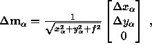 thus
thus
![]() .
Hence,
.
Hence,
![]() ,
where we assume the perturbation in image plane is the same for each point
(with mean zero and standard deviation
,
where we assume the perturbation in image plane is the same for each point
(with mean zero and standard deviation ![]() ).
).
Remark 2: This method is optimal only in the sense of unbiasness. Another criterion of optimality, namely the minimum variance of estimation, is not addressed in this method.