IBM of clonal plant dynamics

An Individual-based model simulator for clonal plant growth developed in 2011 and 2012 in the context of the ANR Syscom project Modecol, in Matlab.

Context

It was developed within the ANR Syscomm (SYStèmes Complexes et Modélisation Mathématique) project MODECOL ( MODélisation ECOLogique de prairies virtuelles) [ANR-08-SYSC-012]. The model presented here is detailed and analyzed in: F. Campillo and N. Champagnat, Simulation and analysis of an individual-based model for graph-structured plant dynamics, Ecological Modeling 2012. [PDF].

Description

We propose a stochastic individual-based model of graph-structured population, viewed as a simple model of clonal plants. The dynamics is modeled in continuous time and space, and focuses on the effects of the network structure of the plant on the growth strategy of ramets. This model is coupled with an explicit advection-diffusion dynamics for resources.

At time $t$ clonal plant is represented as a set of nodes (ramets) that may be connected by links (rhizomes or stolons). In this simplified representation of a clonal plant, ramets are represented by points in the plane, and connection by lines. The state of the nodes is described by the following finite measure:

$\nu_t=\sum_{i=1}^{N_t}\delta_{x^i_t}$

where $x^i_t\in\mathcal{D}$ is position of the $i$ th node and $N_t$ total number of nodes; $\delta$ denotes the Dirac measure centered on the point $x$ . The measure $\nu_t$ describes the distribution of nodes over the space $\mathcal{D}\subset\mathbb{R}^2$ of spatial positions. For any node at position $x$ we define the set of indices of the nodes connected to $x$ :

$J(t,x) = \{i = 1,\dots,N_t; x \textrm{ and }x^i_t \textrm{ are connected} \}\,.$

The plant grows in a resource landscape. At each time $t$ , this resource landscape is represented by $\mathbf{r}(t, x)\geq 0$ the available resources at position $x\in\mathcal{D}$ . The nodes accessing high levels of resources $\mathbf{r}(t, x)$ are more likely to give birth to new nodes.

Birth and death rates

Each node of $\nu_t$ in position $x$ may disappear at a death rate $\mu(t, x)$ and give birth to a new node at a birth rate $\lambda(t, x)$ . These rates are per capita rates. Global death and birth rates at population level are respectively: $\bar\lambda_t=\sum_{i=1}^{N_t}\lambda(t,x^i_t)$ and $\bar\mu_t=\sum_{i=1}^{N_t}\mu(t,x^i_t)$ ; the global event rate is $\bar\lambda_t+\bar\mu_t$ . Basically, the per capita rates depend on the local availability of resources: we suppose that the birth rate $\lambda(t, x)$ is an increasing function of $\mathbf{r}(t, x)$ and the death rate $\mu(t, x)$ is a decreasing function of $\mathbf{r}(t, x)$ . When a node is added to the population, it is always linked with the mother node; when a node $x$ is removed from population, all connections to $x$ are suppressed.

Dispersion kernel

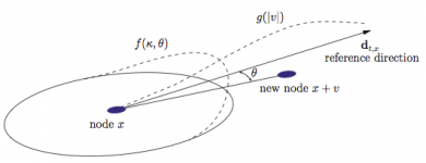
A node at position $x$ at time $t$ gives birth to a new node at position $y = x + v$ according to the p.d.f. $D_{t,x} (v)= f (\kappa, (d_{t,x} , v)),g (|c|)$ . $(d_{t,x},v)$ is the angle between the preferred direction of reference $d_{t,x}$ and the direction of the new shoot $v$ . $f$ is the p.d.f. of the angle of the new shoot and $g$ is the p.d.f. of the length of the associated link. $d_{t,x}$ will be a rough approximation of the gradient of $\mathbf{r}(t,x)$ given by connected nodes.

Interactions between nodes and resources

For the coupling of the (discrete) individual dynamics with the resource density dynamics $\mathbf{r}(t,x)$ is modeled as:

( $\triangle$ ) $\partial_t \mathbf{r}(t,x)=\textrm{div}(\mathbf{a}(x),\nabla \mathbf{r}(t,x))+\mathbf{b}(x)\cdot\nabla \mathbf{r}(t,x)-\alpha,\mathbf{r}(t,x),\sum_{i=1}^{N_t} \Gamma_{x^i_t}(x)  $

we model with the kernel $\Gamma_{x^i_t}(x)$ the fact that resource consumption is not local.

Exact Monte Carlo simulation of the IBM

The only approximation is the numerical integration of the resource dynamics $(\triangle)$ which is performed with a finite difference scheme.

, ,  given
for  do
   compute the rate  and 
   , 
    with 
   if  then
      sample  according to 
      sample  according to 
       [birth]
   else
      sample  according to 
      
   end if
      compute  [numerical approximation of ]
end for

Simulation

Here the angle p.d.f. $f$ is a Von Mises distribution of parameters $\mu_{\textrm{\tiny\rm f}}$ and $\kappa_{\textrm{\tiny\rm f}}$ ; the length p.d.f. $g$ is a log-normal distribution of parameters $\mu_{\textrm{\tiny\rm g}}$ and $\sigma^2_{\textrm{\tiny\rm g}}.$ The maximum link per node is $N_{\text\rm{\tiny\rm links}}$ .

Guerilla

$N_{\textrm{\tiny\rm links}}=3$ , $\mu_{\textrm{\tiny\rm g}}=-1.8$ , $\sigma^2_{\textrm{\tiny\rm g}}=0.1$ , $\mu_{\textrm{\tiny\rm f}}=0$ , $\kappa_{\text\rm{\tiny\rm f}}=400$ :

Phalanx

$N_{\text\rm{\tiny\rm links}}=3$ , $\mu_{\text\rm{\tiny\rm g}}=-2.5$ , $\sigma^2_{\textrm{\tiny\rm g}}=0.1$ , $\mu_{\textrm{\tiny\rm f}}=0$ , $\kappa_{\textrm{\tiny\rm f}}=0.0000000001$ :