Surface registration with LDDMM & currents

The smooth diffeomorphic transformation ϕⁱ that registers the template to the observations ⁱ is estimated using the Large Deformation Diffeomorphic Mappings (LDDMM) method [2, 3, 4] on currents [1, 5]. Diffeomorphic transformations are crucial as they ensure one-to-one mapping between the two shapes. No material loss nor topology changes are allowed, thus guaranteeing the consistency of the analysis. ϕⁱ is obtained by integrating the Lagrangian transport equation ∂ϕⁱ(,t)∕∂t = ⁱ(ϕⁱ(,t),t), ϕⁱ(,t = 0) = . However, the velocity field ⁱ now varies over time, yet completely determined by the initial velocity field ⁱ(,t = 0), denoted ₀() to simplify the notations. As for the currents, the initial velocities ₀ⁱ() belong to a r.k.h.s. V generated by the Gaussian kernel K_V (,) = exp(-∥ -∥²∕λ_V ²). They are thus parameterised by moment vectors βⁱ. Intuitively, the moment vectors contain the initial kinetic energy that is necessary to cover the geodesic path ϕⁱ. For discrete surfaces, the moments are defined at the location _k of the Dirac delta currents. As a result, the initial velocity field verifies ₀ⁱ() = ∑_kK_V (_k,)β_kⁱ. The kernel K_V defines an inner product of the space of velocities V , < ₀ⁱ,₀^j > _V = ∑_k,lβ_k^iT K_V (_k,_l)β_l^j.

The transformation ϕⁱ is estimated by minimising the registration energy defined on the current:

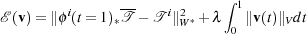(1)

where λ is a weight parameter that controls the strength of the regularisation and ϕⁱ(t = 1)_* is the action of the diffeomorphism at time t = 1 on the template . How this energy is minimised is detailed in [5, 1]. What is important to consider for our application is the effect of the kernel K_V on the estimated deformations. The matching criterion on currents is regularised by minimising the length along the geodesic diffeomorphism, which is computed by integrating the velocity field (t) over time. As an analogy, the length of the geodesic ϕ is the distance that a car would cover between time t = 0 and t = 1 when its instant velocity is (t). The norm of the velocity is computed in the space V , whose members are obtained by convolving the moment vectors with the kernel K_V . Hence, the kernel K_V controls the smoothness of the velocity ₀, and thus of the transformation ϕ. In other words, λ_V ² controls the size of the spatial region that is deformed consistently. When λ_V ² is large, wide spatial regions are deformed in a coherent way, and reversely. Thus, one can control the amount of shape variability to analyse. For studying global shape differences, large λ_V ² are suggested, and conversely.

References

[1]    M. Vaillant and J. Glaunes, “Surface matching via currents,” in Proc. IPMI 2005, p. 381, Springer, 2005.

[2]    P. Dupuis, U. Grenander, and M. Miller, “Variational problems on flows of diffeomorphisms for image matching,” Quaterly of Applied Mathematics, vol. 56, no. 3, pp. 587–600, 1998.

[3]    M. Miller, A. Trouvé, and L. Younes, “On the metrics and Euler-Lagrange equations of computational anatomy,” Annual review of biomedical engineering, vol. 4, no. 1, pp. 375–405, 2002.

[4]    M. Beg, M. Miller, A. Trouvé, and L. Younes, “Computing Large Deformation Metric Mappings via Geodesic Flows of Diffeomorphisms,” International Journal of Computer Vision, vol. 61, no. 2, pp. 139–157, 2005.

[5]    J. Glaunčs, Transport par difféomorphismes de points, de mesures et de courants pour la comparaison de formes et l’anatomie numérique. PhD thesis, Université Paris 13, 2005.