Computational Anatomy of the Brain
3. A Statistical Framework for Anatomical Curves and Surfaces
3.1 Specific Approximation Tools for Groupwise Statistics
As emphasized in Section 1, one the major goal of Computational Anatomy is to compute, process and visualize statistics on large database of anatomical curves or surfaces. As shown on the sulcal lines in Section 2, modeling such geometrical primitives with currents avoids to rely on point-correspondence method between structures, which may introduce bias in the statistical estimation. It also allows to use all the information of the curve or surface without having to chose a priori a reduced set of characteristic measurements (length, area, volume, curvature, etc.). The framework based on currents has been proved to be powerful for pairwise registration of brain surfaces. However, new numerical schemes are required to process groupwise statistics due to an increasing complexity when the size of the database is growing. For example, the registration scheme for currents has a polynomial complexity in the number of points in shapes. In the space of current the mean or the first mode contains as many points as the total number of points within the dataset. Registering the mean shape therefore becomes untractable as the number of instances in the database becomes important (which is what we aim at for good statistics).
To solve that problem, we propose an efficient computational framework that overcomes this limitation by providing a sparse representation of currents at any desired accuracy [Durrleman et al., 2008b]. Actually, the statistics of currents such as mean or principal modes often have a highly redundant representation. Our algorithm builds on ideas from the approximation theory previously developed to decompose images in wavelet bases [Mallat and Zhang, 1993]. To the very best of our knowledge, this is the first time that these signal processing techniques are used in geometric shape analysis. As a result, the method finds an adapted basis, which minimizes in some sense the redundancy of the representation. Besides the computational improvement, this sparse representation offers a way to visualize and interpret statistics on currents. Following experimental results clearly demonstrate the interest of our method.
3.2 Groupwise Statistics on Sets of Curves
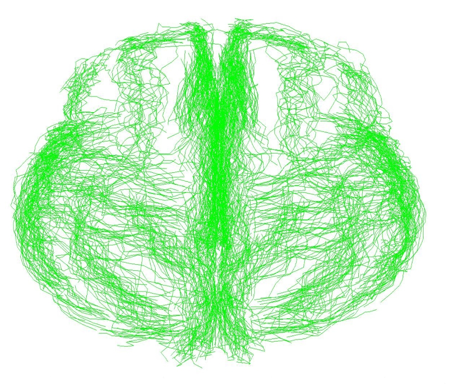
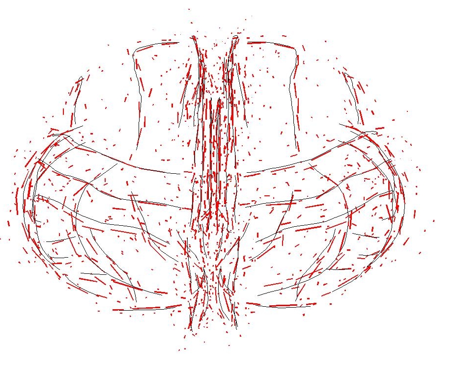
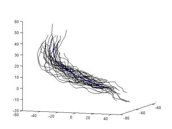
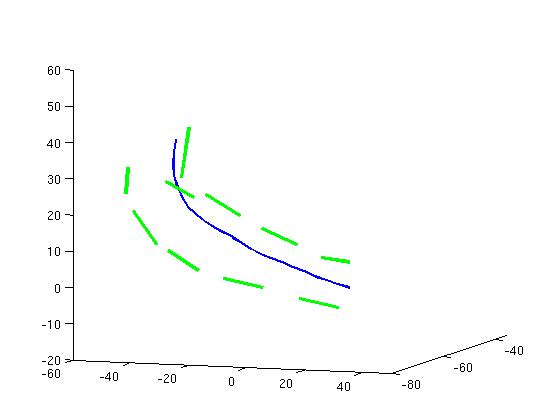
The sulci are the fissures on the brain surface and they are often used to measure anatomical differences between subjects, as emphasized in Section 2. We use here a set of 70 sulci delineated in 34 subjects. For each sulcal line, we give a sparse representation of the mean current with an approximation error below 5% of the variance. Results are shown in Fig. 1 for all 70 sulci. A close-up of the Sylvian Fissure of the right hemisphere is shown in Fig. 2. The initial mean fissure contains 899 segments (i.e. the number of segments of all lines), whereas the final approximation requires only 54 momenta. This gives a compression ratio of 94%. Considering all sulci, the compression ratio is on average: 94.8%. We see also that our mean is in good agreement with other mean curves computing from B-spline representation [Fillard et al., 2007].
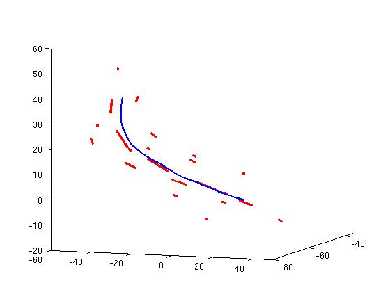
Then, we compute a PCA on the lines set to retrieve its first eigenmodes. The eigenmodes are given as linear combinations of the input currents. We approximate these combinations with an error below 5% of the variance. The first eigenmodes of the Sylvian Fissure of the right hemisphere is shown in Fig. 2. This mode captures mainly the spreading of the lines set.
 |
 |
 |
 |
 |
3.3 Groupwise Statistics on Sets of Surfaces
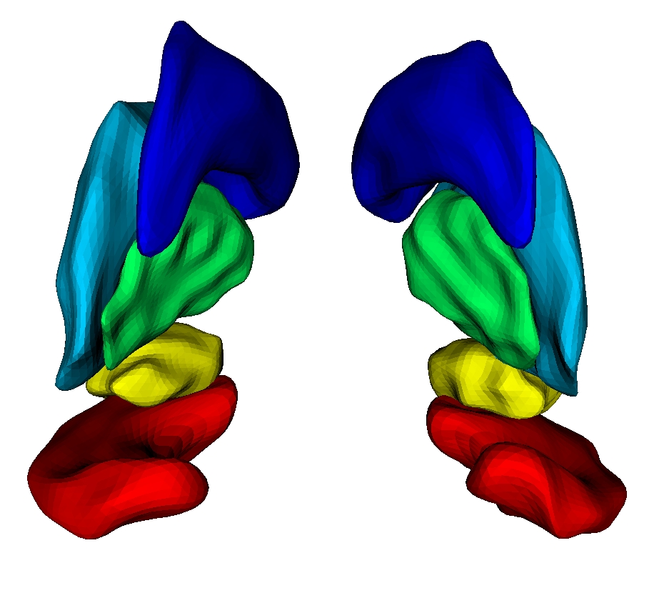
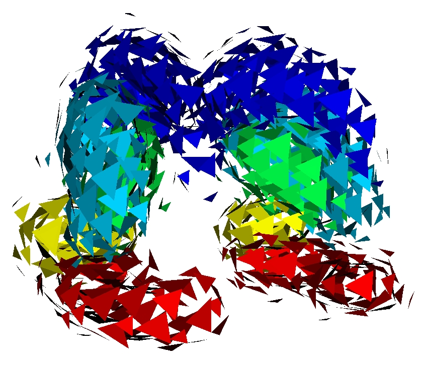
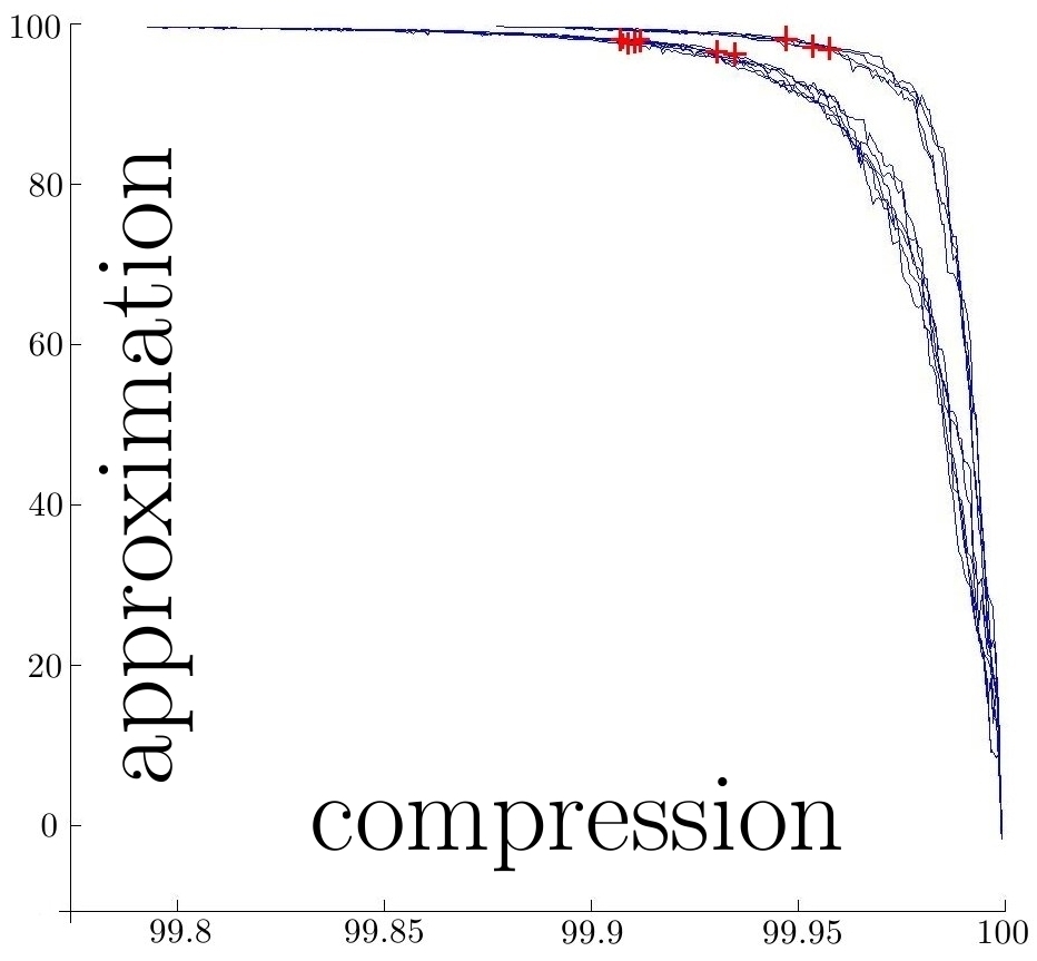
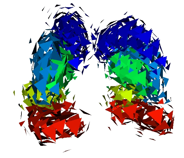
We compute the mean current of 10 meshes of deep brain structures: Caudate, Putamen, Globus Pallidus, Amygdala and Hippocampus for each hemisphere for 50 autistics children of age 2 [Hazlett et al., 2005]. For surfaces, we represent a momenta by a small triangle whose normal is the momenta. Results are shown in Fig. 3. The compression ratio achieved for these 10 surfaces is on average of 99.96%. Representing the mean requires 1.2 Kb in our framework, versus 8 Mb originally. Fig. 3 (right panel) shows that the quality of approximation remains good until very high compression ratio. The deformation of a mean obtained from only 3 shape instances, each with 15 000 points, which was previously taking 10 hours, is now taking about 5 minutes (using the same code as in [Vaillant and Glaunes, 2005; Durrleman et al., 2008a]. For the full set of 50 instances, deforming the former still requires 5 minutes while it is not feasible to deform the later without high performance computing.
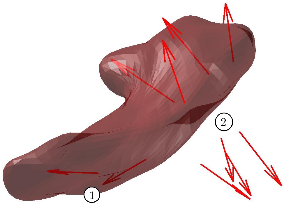
Similarly, we compute mean from meshes of 7 controls. The difference between both means is a current that we approximate: the arrows of Fig.4 are the first 10 estimated momenta of this difference, suggesting that the autistic mean is more curved at the Hippocampus' extremity and thicker in the middle. Such results still need to be confirmed by rigorous statistical tests.
 |
 |
 |
 |
 |
3.4 References
- [Durrleman et al, 2008a] Durrleman S., Pennec X., Trouvé A., Thompson P.M., Ayache N., Inferring brain variability from diffeomorphic deformations of currents: an integrative approach. Medical Image Analysis, 12 (5):626-637, 2008
- [Durrleman et al, 2008b] Durrleman S., Pennec X., Trouvé A., Ayache N., Sparse Approximation of Currents for Statistics on Curves and Surfaces. In Proceedings of Medical Image Computing and Computer Assisted Intervention (MICCAI), Part II, volume 5242 of LNCS, New-York, USA, pages 390-398, Springer (2008).
- [Fillard et al., 2007] Fillard P., Arsigny V., Pennec X., Hayashi K., Thompson P.M., Ayache N., Measuring Brain Variability by extrapolating sparse tensor fields measured on sulcal lines. NeuroImage 34 (2) pages 639-650, 2007
- [Hazlett et al., 2005] Hazlett H., Poe M., Gerig G., Smith R., Provenzale J., Ross A., Gilmore J., Piven J., Magnetic Resonance Imaging and Head Circumference Study of Brain Size in Autism, The Archives of General Psychiatry 62, pages 1366-1376, 2005
- [Mallat and Zhang, 1993] Mallat S., Zhang Z., Matching Pursuits with time-frequency dictionaries, IEEE Transactions on Signal Processing 41 (12), pages 3397-3415, 1993
- [Vaillant and Glaunès, 2005] Vaillant M., Glaunès J., Surface Matching via Currents, Proceedings of Information Processing in Medical Imaging. Volume 3565 of LNCS. Springer (2005)