Computational Anatomy of the Brain
2. Morphometry of the Cortex Inferred from Sulcal Lines
2.1 A point-wise Line Correspondence Approach
In the context of the INRIA-associated team BrainAtlas with Paul Thompson at the Laboratory of Neuro Imaging, University of California at Los Angeles (LONI), we proposed with Pierre Fillard to infer the variability of the brain from a dataset of precisely delineated anatomical structures (sulcal lines) on the cerebral cortex. We model the first- and second-order moments of sulci by an average sulcal curve and a sparse field of covariance tensors along these curves. The covariance matrices are then extrapolated to the whole brain using a harmonic diffusion PDE on the manifold of tensor fields. As a result, we obtain a dense 3D variability map, which proves to be in accordance with previously published results on smaller samples of subjects. Statistical tests demonstrated that our model was globally able to recover some missing information. Preliminary results on the correlation between local and distant displacements indicate that the displacement of the symmetric point is correlated. Other long-distance correlations also appear, but their statistical significance still needs to be established.
2.2 A new Correspondence-less Diffeomorphic Method
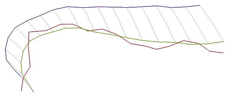
In [Durrleman et al., 2007], we apply a correspondence-less diffeomorphic method on the same dataset of sulcal lines. We kept the same set of mean lines but the model ling of both line matching and deformations is different.Firstly, lines are modelled as currents (see [Vaillant and Glaunès, 2005] for details). The space of currents is a linear space that has many interesting mathematical properties: linear operations (addition and scaling), continuous and discrete lines are handled in the same setting with some convergence properties... . Moreover, can compute a geometric distance between two lines without any assumptions about point to point correspondences . This enables to define a 'probabilistic' line matching criterion which can be optimised to constraint the global space deformation. (see figure 4.) This framework is very general and could be used not only for lines but also for surfaces or volumes.
Secondly, the large deformation framework is rooted in the paradigm of Grenander's group action approach for modelling objects [Grenander 1993, Miller et al, 2006]. The deformations are searched in a subgroup of the group of diffeomorphisms (smooth and invertible mappings). Such deformations are defined in the whole space and act on currents. In the case of curves and surfaces this action coincides with their natural geometrical transportation.
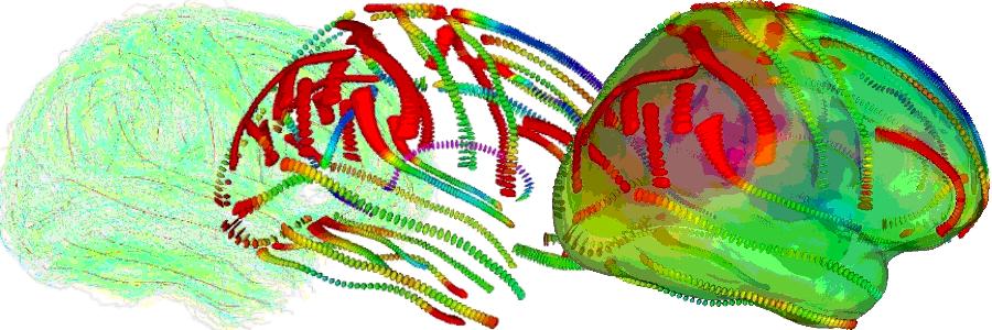
Finally, the registration is found by minimising a cost function that makes a compromise between the regularity of the diffeomorphism and the fidelity to data computed via the distance between currents. In this setting, we do not only find an optimal matching between two lines sets but also recover a global consistent deformation of the underlying biological material on which the lines are drawn. As an example the following video show the registration of a mean brain into a subject's one constrained by the sulcal lines.
This framework has the advantage of being generative. This means that we can compute samples of sulcal lines according to the Gaussian model we have learnt on the data. In particular, we can compute a tangent-PCA on the displacement field and retrieve the different modes of deformations of the database. This gives a description of the major trends of geometrical variations within the studied population. The following video shows the first deformation mode of the database: according to the Gaussian prior, this deformation is the principal trend of variations within the population.
2.3 Comparison of Both Methods
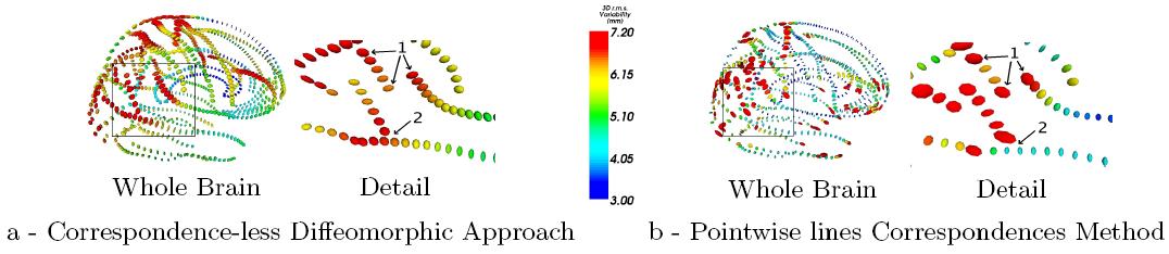
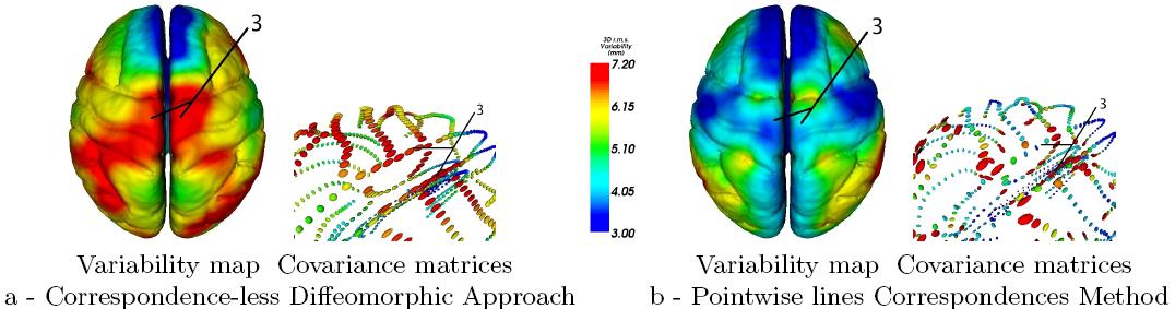
In the correspondence-less diffeomorphic approach (called here CLD) we can take advantage of the tangent space representation of the diffeomorphisms (as in [Vaillant et al, 2004]) to compute similar maps as those obtained by the previous method set up by P. Fillard and based on point-wise lines correspondences (PwLC). These maps of variability enable to emphasise the differences between both approach. These differences are explained by the hypothesis on which each method is based.
Since the CLD's approach 'integrate' the information in a spatially consistent and smooth way, the retrieved variability is naturally more regular. This is particularly visible at lines crossing or between points that belong to different lines as highlighted in figure 5. The modelling based on the currents enables also to give an alternative to the systematically under-estimated tangential variability in the PwLC's approach as explained by the figure 6. Beyond these two obvious differences, a deeper analysis can also be performed to analyse more subtle variations as presented in [Durrleman et al, 2007].
2.4 References
- [Durrleman et al, 2007] Durrleman S., Pennec X., Trouvé A., Ayache N., Measuring Brain Variability via Sulcal Lines Registration: A Diffeomorphic Approach, MICCAI 2007, to appear.
- [Grenander, 1993] Grenander U., General Pattern Theory, Oxford Science Publications, 1993
- [Miller et al, 2006] Miller M., Trouvé A., Younes L., Geodesic Shooting for Computational Anatomy. Journal of Mathematical Imaging and Vision, 2006.
- [Pennec, et al 2005] Xavier Pennec, Radu Stefanescu, Vincent Arsigny, Pierre Fillard, and Nicholas Ayache. Riemannian Elasticity: A statistical regularization framework for non-linear registration. In J. Duncan and G. Gerig, editors, Proceedings of the 8th Int. Conf. on Medical Image Computing and Computer-Assisted Intervention - MICCAI 2005, Part II, volume 3750 of LNCS, Palm Springs, CA, USA, October 26-29, pages 943-950, 2005. Springer Verlag. PMID: 16686051.
- [Pennec, 2006] Xavier Pennec. Left-Invariant Riemannian Elasticity: a distance on Shape Diffeomorphisms?. In X. Pennec and S. Joshi, editors, Proc. of the International Workshop on the Mathematical Foundations of Computational Anatomy (MFCA-2006), pages 1-13, 2006.
- [Vaillant et al, 2004] Vaillant M., Miller M., Younes L., Trouvé., Statistics on diffeomorphisms via tangent space representation, NeuroImage 23, 161-169, 2004
- [Vaillant and Glaunès, 2005] Vaillant M., Glaunès J., Surface Matching via Currents, Proceedings of Information Processing in Medical Imaging. Volume 3565 of LNCS. Springer (2005)