. Complete functional

We compute a packet wavelet decomposition of the image (up to the second order in practice): we get $I$ channels ($I=16$ in practice).

We call the energy at pixel $s$ the vector $U(s)=(U_{1}(s),\dots, U_{I}(s))$, where $U_{i}(s)$ is the square of the wavelet coefficient in the sub-band $i$ at pixel $s$.

Hypotheses:

(H 1) We assume that, for each texture $k=1\dots K$, in each channel $i=1\dots I$, the square of the wavelet coefficients follows a law of the type (4.4).

(H 2) We consider that the different channels are independent.

Data term

We want to maximize $P(U\vert Cl)$, where $Cl$ is the assumed class (Maximum Likelihood Estimator).

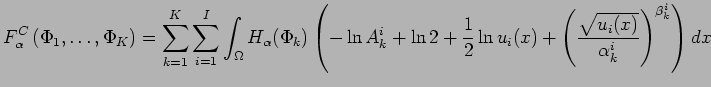
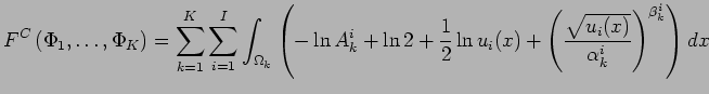
Our fitting term to the data is:

$$F^{C}\left(\Phi_{1},\dots,\Phi_{K}\right)= \sum_{k=1}^{K} \sum_{i... ... \left( \frac{\sqrt{u_{i}(x)}}{\alpha_{k}^{i}} \right)^{\beta_{k}^{i}}\right)dx$$ (5.1)

And 5.1 is given by:

$$F_{\alpha}^{C}\left(\Phi_{1},\dots,\Phi_{K}\right)= \sum_{k=1}^{K... ... \left( \frac{\sqrt{u_{i}(x)}}{\alpha_{k}^{i}} \right)^{\beta_{k}^{i}}\right)dx$$ (5.2)

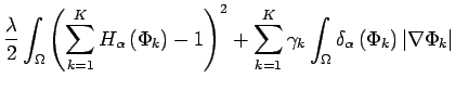
The functional

We are now able to completely write the functional which models the classification problem for textured images:

$$F\left(\Phi_{1},\dots,\Phi_{K}\right) = \frac{\lambda}{2} \int_{\Omega}\left( \sum_{k=1}^{K}H_{\alpha}\le... ...\int_{\Omega} \delta_{\alpha} \left( \Phi_{k} \right) \vert\nabla \Phi_{k}\vert$$ (5.3)

$$+\sum_{k=1}^{K} e_{k} \sum_{i=1}^{16} \int_{\Omega} H_{\alpha}(\P... ... \left( \frac{\sqrt{u_{i}(x)}}{\alpha_{k}^{i}} \right)^{\beta_{k}^{i}}\right)dx$$

Euler-Lagrange Equations

We get the following system composed of $K$-coupled PDE's: we have for $k=1\dots K$

$$0= \lambda \delta_{\alpha}(\Phi_{k}) \left( \sum_{q=1}^{K} H_{\al... ... \frac{\sqrt{u_{k}^{i}}}{\alpha_{k}^{i}} \right)^{\beta_{k}^{i}}\right) \right)$$ (5.4)

Dynamical scheme

To solve the PDE's system (5.4), we embed it in the following dynamical scheme ( $k=1\dots K$):

$$\frac{\partial \Phi_{k}}{\partial t} = -\delta_{\alpha}(\Phi_{k}) \left[ 2 \lambda \left( \sum_{q=1}^{K}... ...a_{k} div\left(\frac{\nabla \Phi_{k}}{\vert\nabla \Phi_{k}\vert}\right) \right.$$

$$\left. +e_{k}\left( \sum_{i=1}^{16} \left( -\ln A_{k}^{i}+ \ln 2 ... ...c{\sqrt{u_{i}(x)}}{\alpha_{k}^{i}} \right)^{\beta_{k}^{i}}\right)\right)\right]$$ (5.5)

with the initial condition $\Phi_{k}(0,x)$ is the Euclidean signed distance function to the zero level set $\Phi_{k}$.

We discretize this system with finite differences.

Reinitialization

The $\Phi_{k}$ are initialized as Euclidean signed distance functions. Nevertheless, as in the classical active contour method, the evolution of the $\Phi_{k}$ with respect to (5.5) does not keep them as Euclidean signed distance functions to their zero level set.

To reinitialize $\Phi_{k}$ into the Euclidean signed distance function, we use the PDE:

$$\frac{\partial \Phi}{\partial t}+sign(\Phi_{k})(\vert\nabla \Phi\vert-1)=0$$ (5.6)