. Classification

Partition, level set approach

The image is considered as a function $u_{0}: \Omega \mapsto {\mathbb{R}}$ (where $\Omega$ is an open subset of ${\mathbb{R}}^2$)

We denote $\Omega_{k}=\left\{x\in \Omega / \mbox{x belongs to the class k}\right\}$. The collection of open sets $\left\{ \Omega_{k} \right\}$ forms a partition of $\Omega$ if and only if

$$\Omega=\bigcup_{k}\Omega_{k}\bigcup_{k} \Gamma_{k}$$    , and if $$k\neq l$$     $$\Omega_{k}\bigcap \Omega_{l}=$$Ø

We denote $\Gamma_{k}=\partial \Omega_{k}\bigcap \Omega$ the boundary of $\Omega_{k}$ (except points belonging also to $\partial \Omega$), and $\Gamma_{kl}=\Gamma_{lk}=\Gamma_{k}\bigcap\Gamma_{l}\bigcap\Omega$ the interface between $\Omega_{k}$ and $\Omega_{l}$ (see figure 1).

Figure 1: Classification seen as a partition problem

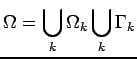
In order to get a functional formulation rather than a set formulation, we suppose that for each $\Omega_{k}$ there exists a lipschitz function $\Phi_{k}:\Omega \rightarrow \mathbb{R}$ such that:

$$\left\{ \begin{array}{ll} \Phi_{k}(x)>0 & \mbox{if $x\in \Omega_{... ...x{if $x\in \Gamma_{k}$}\\ \Phi_{k}(x)<0 & \mbox{otherwise} \end{array}\right.$$

$\Omega_{k}$ is thus completely determined by $\Phi_{k}$.

Regularization

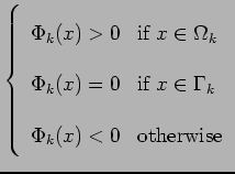
In our equations, there will appear some Dirac and Heaviside distributions $\delta$ and $H$. In order that all the expressions we write have a mathematical meaning, we use the classical regular approximations of these distributions (see figure 2):

Figure 2: Approximations $\delta _{\alpha }$ and $H_{\alpha }$ of the Dirac and Heaviside distributions

$$\delta_{\alpha}=\left\{ \begin{array}{ll} \frac{1}{2\alpha}\left(... ...vert\leq \alpha$} \\ 0 & \mbox{if $\vert s\vert<\alpha$ } \end{array}\right.$$

$$H_{\alpha}=\left\{ \begin{array}{ll} \frac{1}{2}\left(1+\frac{s}{... ... 1 & \mbox{if $s>\alpha$ } \\ 0 & \mbox{if $s<\alpha$ } \end{array}\right.$$

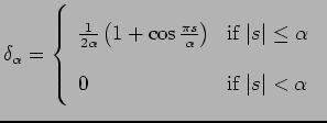
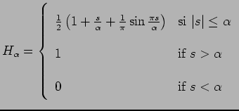
Figure 3 shows how the regions are defined by these distributions and the level sets.

Figure 3: Definitions of the regions and of their level sets

Functional

Our functional will have three terms:

1) A partition term:

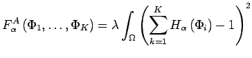$$F_{\alpha}^{A}\left(\Phi_{1},\dots,\Phi_{K}\right)=\lambda \int_{\Omega}\left( \sum_{k=1}^{K}H_{\alpha}\left(\Phi_{i}\right)-1\right)^2$$ (2.1)

2) A regularization term:

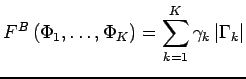$$F^{B}\left(\Phi_{1},\dots,\Phi_{K}\right)=\sum_{k=1}^{K} \gamma_{k} \left\vert \Gamma_{k}\right\vert$$ (2.2)

In practice, we seek to minimize:

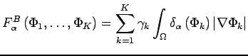$$F^{B}_{\alpha}\left(\Phi_{1},\dots,\Phi_{K}\right)=\sum_{k=1}^{K}... ...\int_{\Omega} \delta_{\alpha} \left( \Phi_{k} \right) \vert\nabla \Phi_{k}\vert$$ (2.3)

3) A data term:

$$F^{C}\left(\Phi_{1},\dots,\Phi_{K}\right)$$ (2.4)

The functional we want to minimize is the sum of the three previous terms:

$$F(\Phi_{1},\dots,\Phi_{K})=F^{A}(\Phi_{1},\dots,\Phi_{K})+F^{B}(\Phi_{1},\dots,\Phi_{K})+F^{C}(\Phi_{1},\dots,\Phi_{K})$$ (2.5)