| Previous : Point processes | Up : Contents | Next : Algorithm |
|
|||||
|
We aim at detecting buildings on a DEM. We propose to first detect
silhouettes of buildings, and then to estimate their 3D shape.
To achieve this, we model silhouettes of buildings by rectangles.
Our goal is then to detect an unknow number of rectangles on the DEM. We define a process of rectangles and we built its energy using two parts.
Working on S, the space representing rectangles, we introduce a
point process with the following density against the reference marked
Poisson point process of intensity vS. 
|
Figure i) The energy defined for configurations of
rectangles
we want to minimize is a ponderation
between two terms.
 and an external field : 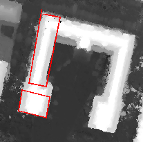 | ||||
|
|||||
|
They are several models available to deal with interactions between
the points of a point process. The simplest one is the pairwise
interaction model. We have done some work to introduce
others model (see [14]) allowing to deal with interactions involving
more than two points. But results presented here were obtained with
simple interactions.
A pairwise interaction model is defined by a symmetric relation
between points ~ , and by an energy under the following form :
 where gamma is a potential function. In the density of point processes section, the relation used was the proximity one, and the potentiel function was equal to V.
Results presented here were obtained using only the intersection
relation
(two rectangles are in interaction iff their intersection is non
empty), and with a potentiel function equal to 1. This makes
intersections be rejected.
|
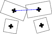
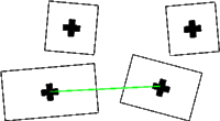
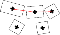
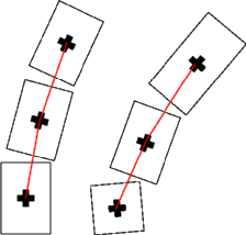
Figure j) We present here some of the interaction that we
have used or tested and the effect of associated potential functions. Proximity Homogeneous close buildings are favourised. 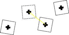
Intersection Intersecting buildings are penalised.
Alignement Aligned buildings are favourised (two or three
points interaction term) with potential functions minimized if
alignement is good and distance between interacting buildings small. | ||||
|
|||||
|
The external part of the energy ensures that the density favourise
silhouettes of builings that are relevant on the DEM.
We use an external field written like :  An other kind of external field can be used. It gives better results, but our algorithm become quite slow while using it. This other external field consist in a distance between the data DEM, and a reconstruction of the DEM made from a configuration of rectangles. Our intensity function uses a ground estimate : for a proposed building, we estimate the heigh of the ground around it. We then look at three different rates, all living in [0,1].
  |
Figure h) We present here how the reward function behave.
is here an extract of a DEM. (by cliquing, you get the third dimension) 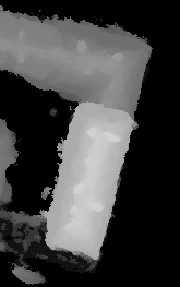
|
| Previous : Point processes | Up : Contents | Next : Algorithm |
