| Main | Introduction | Download Software | Topologies for Assym. resp. |
| About | Tutorial | Dedale registration | Topologies for Symm. resp. |
Dedale-HF is a matlab toolbox dedicated to the “equivalent” network synthesis for microwave filters. It allows, for a given coupling topology and a given filtering characteristic, to compute all possible coupling matrices that will realise the prescribed response with the latter coupling geometry. Whereas for usual canonical topologies, like arrow forms or folded forms, the coupling matrix problem admits a single solution (up to sign changes) it was recently observed [3] that for more general topologies, like extended box ones, the cardinality of the solution set grows rapidly with the filter’s order. For example, for the 10th order extended box topology, there are 384 complex solutions to the coupling matrix synthesis problem. The aim of Dedale is to provide a simple way for designers to perform this coupling matrix synthesis step in an exhaustive manner, i.e. with the guaranty that they do not miss any solution. This exaustivity allows some extra flexibility during the tuning phase an can be used for example to derive some hardware simplifications. It is also of some use when using “coupling matrix identification” procedures [8], [7], [5] and software like Presto-HF during the tuning phase.
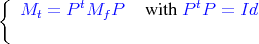
If Mf is a coupling matrix in canonical form of a filtering response Sf the coupling matrix synthesis states as follows [2]: find a similarity transform P and the associated coupling matrix Mt with a prescribed target coupling structure such that:
|
| (1.1) |
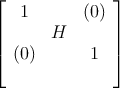
and the similarity transform P has following structure,
Latter conditions guarantee that Mt will give raise to the same response that Mf, provided the same input/output loads are used. Problem 1.1 is in fact a quadratic (non-linear) problem in the entries of P ; indeed if T is the set of indices (i,j) such that in the target topology resonator i and j are not coupled one to another then synthesis problem reduces to:
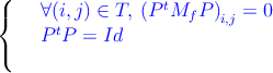 | (1.2) |
Remark: If P0 is a solution of 1.2 then for every sign matrix Δ with following shape,
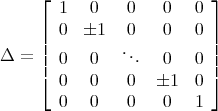
the similarity transform P.Δ is also a solution (the solution set admits a natural sign symmetry).
It can be shown that if the target topology is “non redundant” (i.e do not contain some redundant couplings, see [3] and here for an example) and the original response stays within the set of realisable responses of latter topology then problem 1.2 has finitely many solutions. It is also interesting, that for a given target topology, the number of complex solutions, counted up to sign changes (see prec. remark), will remain the same for almost all possible filtering responses Sf in the realisable set. In other words, for a given topology, the number of complex solutions to the coupling matrix synthesis problem is (generically) independent from the response that is to be synthesized. We call this latter number the reduced order of the coupling topology (reduced, because solutions are counted up to sign symmetries). As opposed to the cardinality of complex solutions the number of purely real ones, which correspond to coupling matrices realisable in practice, varies from one response to another.
Example:
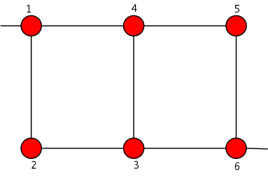
6 poles extended box topology
The reduced order of this topology is 8. It is adapted to the synthesis of asymmetrical responses with up to 2 transmission zeros:
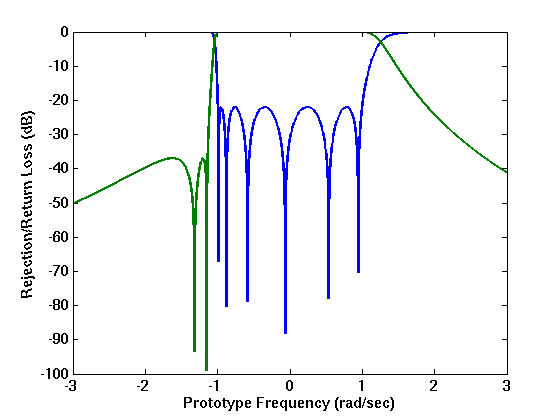
Asymmetrical 6 order response with 2 Tz
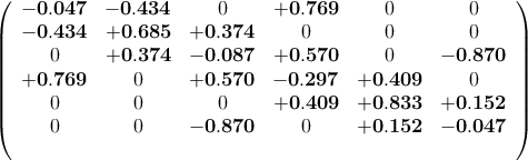
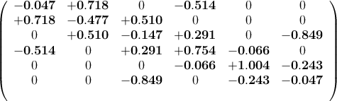
Using Dedale, 8 coupling matrices are computed that realise latter response and 4 of them are found to be purely real:
Input/Output loads: R1 = R2 = 1.089
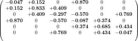
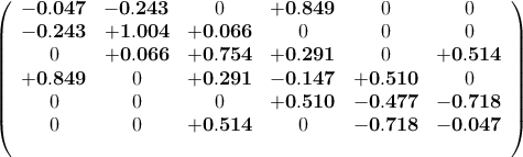
Remark: Note that solution (1) and (3) (resp. ((2) and (4)) are obtained from one another by symmetry through the center of the filter, which is consistent with the fact that optimal quasi-elliptic responses are auto-reciprocal i.e:

For each coupling topology Dedale needs a “reference file” to be able to perform an exhaustive coupling matrix synthesis step. This reference file contains essentially the solution to a particular synthesis problem, i.e all the coupling matrices that realise a particular filtering response. Using this information and continuation techniques, Dedale “transforms” latter solutions to the ones solving the synthesis problem of the user. This can be done because, for a given topology, the mathematical structure of the synthesis problem remains the same. However this structure changes from one topology to the other, and explains why a different reference file is needed for each coupling topology.
Reference files are computed “off-line” in our lab, using computer algebra based techniques and their effective implementations [4], [6], SALSA project. For higher order topologies a numerical method was developed based on the exploration of the monodromy group of an algebraic variety: latter method follows a high number of “paths” in the parameter space and led therefore to the name Dedale !
The Dedale tool is composed of two distinct components:
We plot in what follows a typical Dedale session.
| Main | Introduction | Download Software | Topologies for Assym. resp. |
| About | Tutorial | Dedale registration | Topologies for Symm. resp. |
To work with Dedale you need first to:
Suppose now that you want to synthesize an 8 poles asymmetrical filter with 3 transmission zeros. The synthesis starts classically with the computation of the the polynomials p1 and p2 in terms of which the square modulus of the transmission coefficient expresses as:
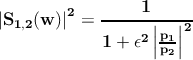
The polynomial p1 is a polynomial built on the reflexion zeros, the
polynomial p2 is built on the transmission zeros, and ϵ is a constant related to
the return loss level (the maximal value of  on the passband is normalized
to 1). For pass-band filter and for fixed transmission zeros, classical formulas
[2], [1] expresses the optimal p1 in the Chebychev sense. In Dedale this can
be done practically by,
on the passband is normalized
to 1). For pass-band filter and for fixed transmission zeros, classical formulas
[2], [1] expresses the optimal p1 in the Chebychev sense. In Dedale this can
be done practically by,
where the first input argument is the order of the response and the second one [-1.35,-1.15, 1.2] is a list of transmission zeros. The passband is implicitly normalized to [-1, 1]. For details about main Dedale functions, use the general help function mechanism from matlab, i.e
We now compute a coupling matrix in canonical form and input/output loads that realise latter elliptic response.
The third argument of latter procedure, i.e 23 here, stays for the desired return loss level. The default canonical form used here is the arrow form, but the folded form is also available with,
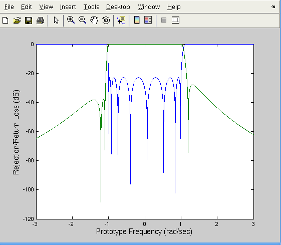
To plot the filter’s response use,
that plots the bode diagram for the frequency range [-3, 3] in the current figure,
Remark: To adjust transmission zeros use the one liner,
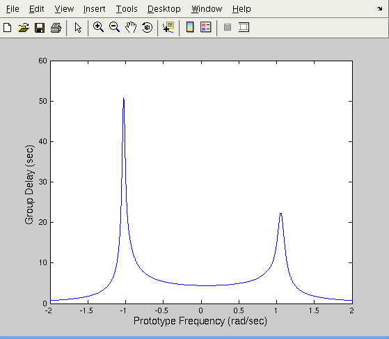
For the group delay diagram, use
to obtain,
For practical implementation, for example with in-line dual mode cavities, neither of the canonical forms is appropriate because of the presence of cross couplings (and for the arrow form, of couplings impossible to realize). We therefore chose a coupling topology out of the database that is compatible with the synthesis of an 8-3 asymmetrical response. This is the case of the form below,
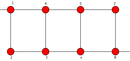
8 poles extended box topology
The reference file can be downloaded from the corresponding web page and after having ’un-gzipped’ it we load it into a matlab reference structure we call ’S’,
The field S.M contains the geometry of the target geometry, and S.LS is the reference solution (list of matrices) already mentioned in preceding section.
To get all complex solutions to the coupling matrix synthesis problem use,
that returns a list of 48 couplings matrices solving the problem. Finally to select the “real solutions”, i.e coupling matrices realisable in practice, use:
that returns 16 coupling matrices that can be used to implement the original response. The second argument for the function ’SelectRealOnes’ is a tolerance parameter: for numerical reasons, real matrices are selected up to a tolerance on the maximum value of the imaginary part of their elements (1e-5 is the default value).
Now starts the job of the designer; depending on the hardware architecture that is intended for the filter one can rank the different coupling matrices. For example in the case of dual mode cavities coupled by irises, one could select here the 12th matrix that has the most asymmetrical irises (i.e ratio between arms dimensions, see [3]) in order to minimize parasitic couplings,
An other choice is to simplify a cross iris by a simple iris, by looking for matrices where iris-couplings are small enough to neglect. This is the case of the 14th matrix,
where the (3, 6) coupling is small enough to neglect. Lots of other criterion can be thought of and we encourage users to program their own ranking procedures depending on the kind of hardware that is used for the filter’s realisation.
[1] S. Amari. Synthesis of cross-coupled resonator filters using an analytical gradient-based optimization technique. IEEE Transaction on Microwave Theory and Techniques, 48(9):1559–1564, 2000.
[2] R. J. Cameron. General coupling matrix synthesis methods for chebyshev filtering functions. IEEE Transaction on Microwave Theory and Techniques, 47(4):433–442, 1999.
[3] R.J. Cameron, J.C. Faugere, and F. Seyfert. Coupling matrix synthesis for a new class of microwave filters. Proceedings of the International Microwave Symposium 2005, Long Beach, 2005.
[4] J.C. Faugere. A new efficient algorithm for computing groebner bases without reduction to zero (f5). Proceedings of the 2002 International Symposium on Symbolic and Algebraic Computation; New York, NY, pages 75–83, 2002.
[5] A. Garcia-Lamperez, S. Llorente-Romano, M. Salazar-Palma, and T.K. Sarkar. Efficient electromagnetic optimization of microwave filters and multiplexers using rational models. IEEE Transaction on Microwave Theory and Techniques, 52:508 – 521, 2004.
[6] L. Gonzalez-Vega, F. Rouillier, and M.F Roy. Symbolic recipes for polynomial system solving. In Some tapas of computer algebra, volume 4 of Algorithms Comput. Math. Springer, Berlin, 1999.
[7] K. Krohne and R. Vahldieck. On the application of model-order reduction in the fast and reliable optimization of microwave filters and diplexers. IEEE Transaction on Microwave Theory and Techniques, 52:2285 – 2291, 2004.
[8] Fabien Seyfert, Jean Paul Marmorat, Laurent Baratchart, Stephane Bila, and Jacques Sombrin. Extraction of coupling parameters for microwave filters: Determination of a stable rational model from scattering data. Proceedings of the International Microwave Symposium, Philadelphia, 2003.