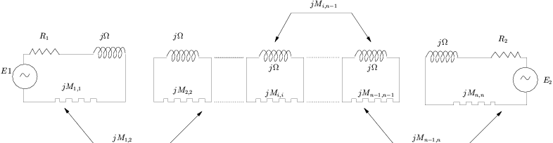
Figure 1.1: Low-pass prototype
| Main | Introduction | Download Software | Topologies for Assym. resp. |
| About | Tutorial | Dedale registration | Topologies for Symm. resp. |
This short tutorial intends to give the key ideas to synthesize a coupling matrix when starting from a rational scattering matrix S and can be seen as a mathematical résumé of R.Cameron’s original paper [3]. In the language of electrical engineering this procedure is called the realization step because it actually computes concrete electrical values in order to implement, by means of a circuit, a specified response. In our case the circuit is the low pass prototype 1.1 and the target response to realize will be given by a specified scattering matrix, i.e. a 2 × 2 rational matrix S of given MacMillan degree n. In this tutorial the particular topology of the coupling matrix, i.e. the way resonators are coupled to one an other, will not be specified; this can be done in a second step and is typically addressed by tools like Dedale-HF (see following tutorial ).
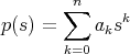
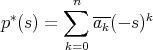
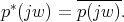
 is a rational function (quotient of two polynomials) then
R* =
is a rational function (quotient of two polynomials) then
R* = 
As we include no resistive elements in our low pass prototype we will start from a loss-less scattering matrix. Such an element S verifies,
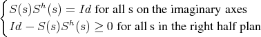 | (1.1) |
Remark: The operator ≥means here positive in the matrix sense.
It can be shown that 2 × 2, degree n, loss-less, symmetrical (S1,2 = S2,1) rational matrices with the identity as a value at infinity admit following general form:
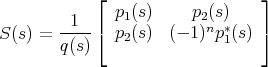 | (1.2) |
with,
 | (1.3) |
For reasons that will become clear later we will suppose moreover that deg(p2) < n - 1.
Latter structure of S (1.2) is a direct consequence from the the lossless property; one easily verifies that with this definition, on the imaginary axes:
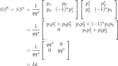 | (1.4) |
The fact that S verifies also the second condition in (1.1) is a consequence of its analyticity (q has its roots in the left half plan) and of the maximum principal.
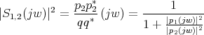
As a consequence S is entirely determined by its numerators p1 and p2, its denominator q being computed from the latter through spectral factorization (1.3). The situation is even simpler for the modulus of elements of S: a straightforward computation yields,

The admittance matrix is defined as the Cayley transform of S,
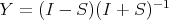
and its elements can be computed from p1, p2 and q
 | (1.5) |
Remark: Latter formulas are equivalent to the expressions given in Cameron’s paper at equations 19 and 20. In his notations for n even we have for example
 | (1.6) |
where (p1)k means the kth coefficient of polynomial p 1.
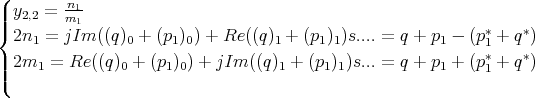
Being the admittance matrix of a lossless system Y verifies,
 | (1.7) |
which is the counterpart for admittances of the relations (1.1). It is a well known fact that lossless admittances have all their poles lying on the imaginary axes. To see this remark that Y has no poles in the right half plan for otherwise it would violate the second relation in (1.7). Now the first relation in (1.7) is equivalent to

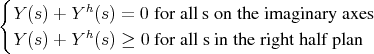
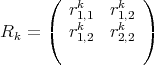
An other well known property that can be deduced from (1.7) is that the poles of a lossless admittance matrix are simple and if,
 | (1.8) |
is the partial fraction expansion of Y then the residues verifies
 | (1.9) |
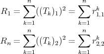
In our case the residues are by construction symmetric i.e Rk = Rkt which combined with (1.9) implies that each Rk is a real, symmetric and non-negative matrix.
Classical realization theory now indicates [4] that if a transfer function Y has simple poles, in other words admits an expansion like (1.8), then
which, under the generic assumption that in (1.5) no pole zero cancelation occures, yields in our 2 × 2 case,

Finally remark that our assumption deg(p2) < n - 1 yields,

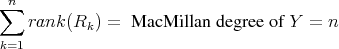
For short the admittance matrix Y computed from S via formulas (1.5) admits a partial fraction expansion of the form (1.8) in which the residues
verifies following property,
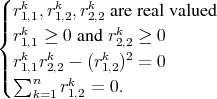 | (1.10) |
and therefore can be factored as
 | (1.11) |
where Tk is the line vector,
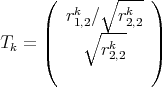
Remark: The latter correspond to expression (A7) in Cameron’s paper
Now if C is the (2 × n) matrix composed of the concatenated Tk vectors (C = (T1,T2...Tn)) and Δ the diagonal (n×n) matrix defined by Δi,i = jwi then expansion (1.8) rewrites as,
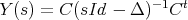 | (1.12) |
Any pair of a (2 ×n) and (n×n) matrices such that (1.12) holds is called a realization of Y . The pair (C, Δ) we just constructed is for example a realization of Y where the matrix of the dynamic (the second matrix in the realization’s pair) is diagonal.
Starting from the low pass prototype (1.1) and applying Ohm’s law one can also derive a realization of Y in terms of the electrical parameter of the network. If M is the coupling matrix of the network, R1,Rn the input/output loads then,
 | (2.1) |
with
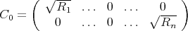 | (2.2) |
In order to be able to identify a coupling matrix and loads we therefore need to transform the realization obtained in (1.12) into a realization in “physical” shape as above. To do so remark that if (F,A) is a realization of Y , i.e.
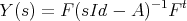 | (2.3) |
and P a similarity transform (PtP = Id) of size n × n then (FP,PtAP) is also a realization of Y . Verification of this is straight forward,
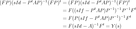 | (2.4) |
If moreover A is symmetric then PtAP is also symmetric.
This is all we need for our purposes. We define P to be any similarity transform having as first and last column vectors the normalized row vectors of C. This is possible because last property in (1.10) indicates that later two vectors are orthogonal. Remark now that the realization (CP,PtΔP) is in “physical shape” meaning that CP only has non-zero elements in the (1, 1) and (2,n) position and that PtΔP is a symmetric pure imaginary matrix and can be interpreted as a coupling matrix. The latter yields in particular,
 | (2.5) |
In practice to obtain the n - 2 missing vectors of P one can first construct a base of the orthogonal complement of the vector space spanned by the row vectors of C and then transform the latter in an orthonormal one using Gram-Schmidt. The latter procedure does not yield a unique determination of the n - 2 missing vectors (as soon as n > 3), and different choices of the base, will yield different coupling matrices. In a tutorial to come we will explain how to avoid latter procedure and directly derive a coupling matrix in the canonical arrow form.
[1] S. Amari. Synthesis of cross-coupled resonator filters using an analytical gradient-based optimization technique. IEEE Transaction on Microwave Theory and Techniques, 48(9):1559–1564, 2000.
[2] S. Bila, R.J. Cameron, V. Lunot, and F. Seyfert. Chebychev synthesis for multi-band filters. Proceedings of the International Microwave Symposium 2006, San Fransisco, 2006.
[3] R. J. Cameron. General coupling matrix synthesis methods for chebyshev filtering functions. IEEE Transaction on Microwave Theory and Techniques, 47(4):433–442, 1999.