To load these data, go to the samples directory and execute:
$ vigie ex_m3d.desc
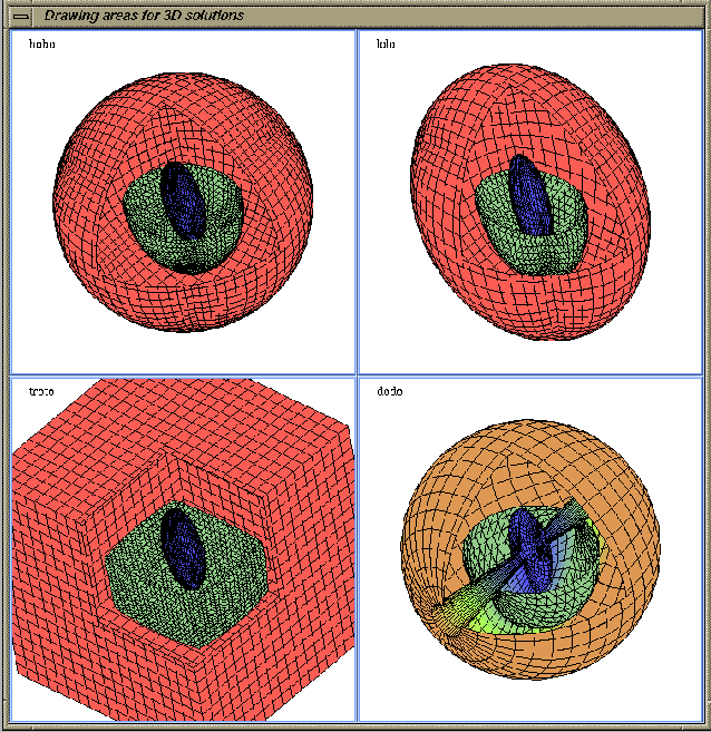
All the interactions needed in usual case are avoided here, by the use of special commands in the description file describe in the section ``extended description files''. You can see, after the time needed for loading the data and executing operations describe in the descrioption file, the picture represented by the figure 1.25.
Content of the description file ``ex_m3d.desc'' follows:
 set_pb_name les_zozos
 set_sol_name bobo
 get_desc ./grosbobo.desc
 set_sol_name lolo
 get_desc ./dulolo.desc
 set_sol_name troto
 get_desc ./patroto.desc
 set_sol_name dodo
 get_desc ./faidodo.desc
 activate_m3d
 set_m3d_drawing_areas on
 set_m3d_toggle global_bb off
 set_m3d_toggle isos off
 set_m3d_toggle csurf on
 set_m3d_toggle mesh on
 set_m3d_toggle ivalue on
 set_m3d_toggle painter on
 add_m3d_plane x.equ.0 1 0 0 0
 add_m3d_plane y.equ.0 0 1 0 0
 add_m3d_plane z.equ.0 0 0 1 0
 m3d_plane x.equ.0 compute_cut all_values
 m3d_plane y.equ.0 compute_cut all_values
 m3d_plane z.equ.0 compute_cut all_values
 comp_m3d_surf cfr2 pos_pcut comp_fr x.equ.0
 comp_m3d_surf cfr3 pos_pcut comp_fr y.equ.0
 comp_m3d_surf cfr4 pos_pcut comp_fr z.equ.0
 add_m3d_isosurf rho001 rho 5.
 m3d_isosurf rho001 compute all_values
 comp_m3d_surf cs30 pos_pcut rho001 x.equ.0
 set_m3d_rot -132. 40. -80.
In the first lines, you can see how you can use other simple description files to insert known data as differents solutions of the same problem. Just after the visualization context for ``multi 3d plot'' is loaded and some toggles are set on or off. After that, three planes are defined, the computed frontier is intersected by these planes, an isosurface is computed and intersected by one of theses planes. In this example, you can see that kind of operations can be defined in a description file, to have more informations on theses features, look at the section ``extended description files''.