Standard Kalman Filter

  When is a linear function

and we are able to write down explicitly a linear relationship

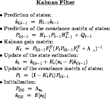
from , then the standard Kalman filter is directly applicable.

  
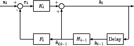
Figure 3: Kalman filter block diagram

Figure 3 is a block diagram for the Kalman filter. At time , the system model inherently in the filter structure generates , the best prediction of the state, using the previous state estimate . The previous state covariance matrix is extrapolated to the predicted state covariance matrix . is then used to compute the Kalman gain matrix and to update the covariance matrix . The system model generates also which is the best prediction of what the measurement at time will be. The real measurement is then read in, and the measurement residual  (also called innovation)

is computed. Finally, the residual is weighted by the Kalman gain matrix to generate a correction term and is added to to obtain the updated state .

The Kalman filter gives a linear, unbiased, and minimum error variance recursive algorithm to optimally estimate the unknown state of a linear dynamic system from noisy data taken at discrete real-time intervals. Without entering into the theoretical justification of the Kalman filter, for which the reader is referred to many existing books such as [8, 14], we insist here on the point that the Kalman filter yields at an optimal estimate of , optimal in the sense that the spread of the estimate-error probability density is minimized. In other words, the estimate given by the Kalman filter minimizes the following cost function

where M is an arbitrary, positive semidefinite matrix. The optimal estimate of the state vector is easily understood to be a least-squares estimate of  with the properties that [4]:

1. the transformation that yields from is linear,
2. is unbiased in the sense that ,
3. it yields a minimum variance estimate with the inverse of covariance matrix of measurement as the optimal weight.

By inspecting the Kalman filter equations, the behavior of the filter agrees with our intuition. First, let us look at the Kalman gain  . After some matrix manipulation, we express the gain matrix in the form:

 

Thus, the gain matrix is ``proportional'' to the uncertainty in the estimate and ``inversely proportional'' to that in the measurement. If the measurement is very uncertain and the state estimate is relatively precise, then the residual is resulted mainly by the noise and little change in the state estimate should be made. On the other hand, if the uncertainty in the measurement is small and that in the state estimate is big, then the residual contains considerable information about errors in the state estimate and strong correction should be made to the state estimate. All these are exactly reflected in (20).

Now, let us examine the covariance matrix of the state estimate. By inverting and replacing by its explicit form (20), we obtain:

 

From this equation, we observe that if a measurement is very uncertain ( is big), the covariance matrix will decrease only a little if this measurement is used. That is, the measurement contributes little to reducing the estimation error. On the other hand, if a measurement is very precise ( is small), the covariance will decrease considerably. This is logic. As described in the previous paragraph, such measurement contributes considerably to reducing the estimation error. Note that Equation (21) should not be used when measurements are noise free because is not defined.