![\[ \left\{ \begin{array}{l} f_1 (x_1, \ldots, x_n) = 0\\ \vdots\\ f_s (x_1, \ldots, x_n) = 0 \end{array} \right. \]](form_367.png)
We consider here the problem of computing the solutions of a polynomial system
in a box ![$I : = [a_1, b_1] \times \cdots \times [a_n, b_n] \subset \mathbbm{R}^n$](form_368.png) . This solver uses the representation of multivariate polynomials in the Bernstein basis, analysis of sign variations and univariate solvers to localise the real roots of a polynomial system. The output is a set of small-enough boxes, which may contain these roots.
. This solver uses the representation of multivariate polynomials in the Bernstein basis, analysis of sign variations and univariate solvers to localise the real roots of a polynomial system. The output is a set of small-enough boxes, which may contain these roots.
By a direct extension to the multivariate case, any polynomial ![$f (x_1, \ldots, x_n) \in \mathbbm{R} [x_1, \ldots, x_n]$](form_369.png) of degree
of degree  in the variable
  , can be decomposed as:
![\[ f (x_1, \ldots, x_n) = \sum_{i_1 = 0}^{d_1} \cdots \sum_{i_n = 0}^{d_n} b_{i_1, \ldots, i_n} \hspace{0.25em} B_{d_1}^{i_1} (x_1 ; a_1, b_1) \cdots B_{d_n}^{i_n} x (x_n ; a_n, b_n) . \]](form_370.png)
where  is the tensor product Bernstein basis on the domain and
  are the control coefficients of
  on
on  . The polynomial is represented in this basis by the
  order tensor of control coefficients
  . The size of , denoted by
  , is
, is  .
.
De Casteljau algorithm also applies in each of the direction , ,  so that we can split this representation in these directions. We use the following properties to isolate the roots:
Definition: For any ![$f \in \mathbbm{R} [ \mathbf{x}]$](form_378.png) and and  , let , let
|
Theorem: [Projection Lemma] For any  , and any , we have , and any , we have
|
As a direct consequence, we obtain the following corollary:
Corollary: For any root  of the equation of the equation  in the domain , we have in the domain , we have  where where
|
The solver implementation contains the following main steps. It consists in
As we are going to see, we have several options for each of these steps, leading to different algorithms with different behaviors, as we will see in the next sections. Indeed the solvers that we will consider are parameterized by the
equivalent to solving the system  , where
  is an
is an  invertible matrix
As such a transformation may increase the degree of some equations, with respect to some variables, it has a cost, which might not be negligible in some cases.
Moreover, if for each polynomials of the system not all the variables are involved, that is if the systems is sparse with respect to the variables, such a preconditioner may transform it into a system which is not sparse anymore. In this case, we would prefer a partial preconditioner on a subsets of the equations sharing a subset of variables.
The following preconditioners are curently avialable:
 .
. , we transform locally the system
  into a system
  , where
  is the Jacobian matrix of at a point
  of the domain , where it is invertible. A direct computation shows that locally (in a neighborhood of
  the level-set of
 are orthogonal to the -axes: This transformation was also discussed in {{gs-isbaspe-01}}. We can prove that the reduction based on the polynomial bounds
  and behaves like Newton iteration near a simple root, that is we have a quadratic convergence.
can be considered.
 and
and  instead of these polynomials., (resp.
  ), in the interval
 ![$[a_j, b_j]$](form_390.png) . The current implementation of this reduction steps allows us to consider the convex hull reduction, as one iteration step of this reduction process. and and keep the intervals
. The current implementation of this reduction steps allows us to consider the convex hull reduction, as one iteration step of this reduction process. and and keep the intervals ![$[ \underline{\mu}, \overline{\mu}]$](form_406.png) defined in corollary [*] ., is achieved by controlling the rounding mode of the operations during the de Casteljau computation.
defined in corollary [*] ., is achieved by controlling the rounding mode of the operations during the de Casteljau computation.This method will be particularly interesting in the cases where more than one interval have to be considered. This may happen at the beginning of the search but is less expected locally near a single root.
subdivide a domain. We will show in the next section their impact on the performance of the solver
is then split in half in a direction  for which
  is maximal. and a
  such that
  (or the difference between the control coefficients) is maximal. Then, a value
  for splitting the domain in the direction
  , is chosen
 has a local maximum,
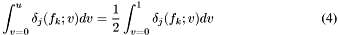
The right-hand side of this equation can be easily computed, from the sum of all the control coefficients of  .
.
synaps/msolve/sbdslv.h.![]()
![]()
#include <synaps/init.h>
#include <synaps/mpol.h>
#include <synaps/base/Seq.h>
#include <synaps/msolve/sbdslv.h>

typedef MPol<double> mpol_t;

int main (int argc, char **argv)
{
  using std::cout; using std::endl;

  mpol_t p("x0^2*x1-x0*x1-1"), q("x0^2-x1^3-2");

  std::list<mpol_t> I; I.push_back(p); I.push_back(q);

  VectDse<double> dmn(4,"-2 2 -2 2");
  //  cout << solve(I, SBDSLV<double,SBDSLV_RDL>())<<endl;
  cout << solve(I, SBDSLV<double,SBDSLV_RDL>(1e-3),dmn)<<endl;

  //| [[1.66068,0.911523], [-1.4228,0.290084]
  //
  // The result is a sequence of vectors with coefficients of double type.
  // The size of the vectors is the number of variables.
  // Here there are no solutions in the default [0,1]x[0,1] and
  // 2 real solutions in the box [-2,2]x[-2,2]).

}
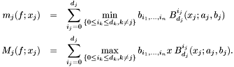
![\[ m (f ; u_j) \le f ( \mathbf{u}) \le M (f ; u_j) . \]](form_382.png)
 (resp.
  ) is either a root of
  or
or  in
in  (resp.
  ) if
) if  on
on ![$[ \underline{\mu}_j, \overline{\mu}_j]$](form_394.png) .
.