
Pascal Cachier, Xavier Pennec
INRIA - EPIDAURE Project, 2004 route des Lucioles, F-06902 Sophia Antipolis
{Pascal.Cachier, Xavier.Pennec}@sophia.inria.fr

In the context of this paper, the goal of non-rigid registration is the retrieval of the motion that has occurred between two volumetric images of the same organ. Because we are working on two images I and J, we have to rely on features of these images. Then, the registration process consists in finding a transformation T that matches well the features, with the hope that these features are significant enough to justify the assumption ``features are matched hence homologous physical points are matched.'' Numerous features are possible, such as points, curves, or intensity. In this paper, we focus on intensity-based methods.
When the intensity is conserved during the motion, an appropriate similarity energy1 is the sum of square differences (SSD). Its gradient is easy to compute and has been used as the guiding force of numerous non-rigid registration techniques [1,2,3,4]. When this assumption is invalid, for example with magnetic resonance images (MRI) corrupted by a non-uniform bias, we have to use more complex criterions, such as the sum of local correlation coefficients (LCC). In this case, the minimization is usually done by a block matching technique using an exhaustive search [5,6,7,8] or a 0th-order minimization strategy [9]. Both the computation of statistics in each hard block and the search of the minimum are computationally intensive for volumetric images. As a consequence, windows are usually sparse and the minimization is done for translations only.
In this paper, we propose to use an isotropic Gaussian window instead of a hard block for the computation of local statistics. This way, we can compute the criterion and its derivatives at each voxel by global convolutions, in a time independent of the extension of the Gaussian window, thus obtaining dense force fields. Section 2 presents the method used to compute local statistics with Gaussian convolutions. Section 3 presents our two-step non-rigid gradient descent based registration algorithm. Finally, we present results of the algorithm on synthetic and real images in Section 4 and we compare different optimization strategies.
When the intensity conservation hypothesis that drives numerous mono-modal non-rigid registration algorithms is violated in medical images, this is mainly due to a non-uniform bias that affects the imaging modality. Therefore, the use of local statistics, and particularly local correlation coefficients, has been increasingly popular. It has even been suggested that it could drive a multi-modal registration [10].
Most of the time, these statistics are computed in a window. The image is divided in some number of square windows that may, or may not, overlap. In its simplest form, the block matching scheme consists in moving each window into several positions, computing a local similarity energy inside the window, and keeping the position of the window leading to the best match. However, it is costly to compute the similarity energy for every position of the window. Hence there is a trade-off between precision and computation time. Generally, one chooses fewer windows than voxels. Also, the motion of the window is often restricted to translation, because adding rotation will multiply the number of estimations, especially in 3D images.
Let
G<B>p be a window function centered around a voxel
pobtained by translation of a discrete, normalized, symmetric kernel
G, and I and ![]() be the two images defined on
be the two images defined on
![]() to
register with a transformation T. We define the local mean of I,
the local correlation between I and
to
register with a transformation T. We define the local mean of I,
the local correlation between I and ![]() ,
the local variance
of I, and the local correlation coefficient between I and
,
the local variance
of I, and the local correlation coefficient between I and ![]() (all of them centered around
p) respectively by:
(all of them centered around
p) respectively by:
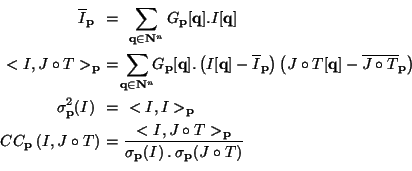
The use of the correlation coefficient enables to compute a distance between two images that is invariant by an affine rescaling of the intensity range on one of the images. It is therefore insensitive to a uniform bias and a linear contrast change.
Because we use local correlation coefficients, the estimation of the bias is done locally. The assumption implicitly done is that the bias should not vary too much inside the window in which the local correlation coefficient is computed. However, the bias is allowed to vary within the image. Hence, we are able to tackle non-uniform biases. We will show later that the LCC criterion (Eq. 1) can actually tackle a bias with a variation up to 50% of the intensity range.
The locality of the correlation coefficients is obtained by
introducing a Gaussian weight (or Gaussian window) in the formulas.
The Gaussian window fulfills two theoretical needs. The first one is
the isotropy2 of the window. Hence, if we compute some
statistics around a point
p, the influence of another point
![]() on the results depends only on its distance to
p. The
second one is the gradual decrease of the influence of remote points.
Remote points should have less influence than points located near the
center of the window. This has some similarity with [11],
where the correlation criterion is not locally weighted but the images
are decomposed onto an Hermite orthogonal basis.
on the results depends only on its distance to
p. The
second one is the gradual decrease of the influence of remote points.
Remote points should have less influence than points located near the
center of the window. This has some similarity with [11],
where the correlation criterion is not locally weighted but the images
are decomposed onto an Hermite orthogonal basis.
Finally, we compute local correlation coefficients around every voxel, and not only a subset of the voxels. Thus, we do not have any privileged point or location in our images, and our measure is invariant by any integer translation.
Fortunately, we are able to compute the local statistics and their
derivatives at a relatively low computational cost, because the
windows are not treated separately but at once, using convolutions.
Using the notations previously introduced, local statistics around
every voxels can be computed altogether with one or two Gaussian
convolutions (denoted by G*):

Because we use Gaussian windows, the derivatives of the criterion can be easily computed using some more Gaussian convolutions. For instance, we put in Table 1 the derivative of the sum of local correlation coefficients criterion with respect to the transformation T[p] of a point p (Eq. 2). We also derived an approximation of the previous formula, where all final convolutions are dropped, in order to be faster (Eq. 3 in Table 1).
In the following, the gradient descent using formula (2) is called Local Correlation Coefficients (LCC). The one using formula (3) is called Simplified Local Correlation Coefficients (SLCC).
 |
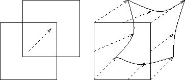
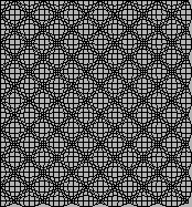
We compute a gradient with respect to the displacement of each voxel. Hence, we have a dense vector field. The first advantage of doing so is that we can handle local, subtle deformations, independently of the spread of the Gaussian used to compute local statistics. A second advantage is that the local similarity of the two images is computed using the real image of the window3 and not its rigid or translational approximation (Fig. 1).
 |
A mathematical equality may hide numerical problems. For example,
consider this equality for the local variance:
![]() .
Whereas the left-hand side will only sum
positive and relatively small numbers, the right-hand side will
compute two big yet close numbers,
.
Whereas the left-hand side will only sum
positive and relatively small numbers, the right-hand side will
compute two big yet close numbers,
![]() and
and
![]() ,
and
then subtract them: we lose several bits of precision. To quantify the
loss of precision, we have compared the results computing the local
variances of the image 2(a) using the left-hand side and using the
right-hand side. We have used real numbers coded on 4 bytes, and as a
preprocessing we have subtracted the mean of the whole image. It
appears that the error in the computation of the local variance using
the difference of mean relatively to the accurate method has an
average of 0.14%
,
and
then subtract them: we lose several bits of precision. To quantify the
loss of precision, we have compared the results computing the local
variances of the image 2(a) using the left-hand side and using the
right-hand side. We have used real numbers coded on 4 bytes, and as a
preprocessing we have subtracted the mean of the whole image. It
appears that the error in the computation of the local variance using
the difference of mean relatively to the accurate method has an
average of 0.14%![]() 0.83% and a median error of 0.00033%. This
means that we have a good numerical precision everywhere, except for
strong outliers which appear to lie on the borders. They are due to
the conjugate effects of the very low variance on these plain black
regions, and the boundary effects of the filter. They are mostly less
than 1%, but reach up to 40% in the 4 corner pixels.
0.83% and a median error of 0.00033%. This
means that we have a good numerical precision everywhere, except for
strong outliers which appear to lie on the borders. They are due to
the conjugate effects of the very low variance on these plain black
regions, and the boundary effects of the filter. They are mostly less
than 1%, but reach up to 40% in the 4 corner pixels.
In our experiments, these errors never had a meaningful incidence on the results, but we should be aware that it can potentially induce some significant distortions in the deformation field at the image borders.
Non-rigid registration using free form transformations is an ill-posed problem that needs regularization. Within the medical image registration community, regularization is often done by choosing a smoothing energy in addition to the similarity energy, and by minimizing both together. Of course, there is a trade-off between the similarity energy, reflected by the visual quality of the registration, and the smoothing energy, reflected by the regularity of the transformation (the term ``regularity'' should be taken in its broadest sense, since the smoothing energy may allow occasional discontinuities in the displacement field [14]). Therefore, we show the result of a non-rigid registration using the deformed image and the transformation itself.
In the regularization theory framework, one minimizes a weighted sum
of both energies
![]() ,
E1 and E2 being
respectively the similarity and the smoothing energies, and
,
E1 and E2 being
respectively the similarity and the smoothing energies, and ![]() being a trade-off coefficient. This formulation has proven to be
successful for data approximation, and has been used for various
approaches of non-rigid registration algorithms
[14,15].
being a trade-off coefficient. This formulation has proven to be
successful for data approximation, and has been used for various
approaches of non-rigid registration algorithms
[14,15].
Another widely used method attempts to separate the image measure from the transformation measure, and could be compared with the approach of game theory. It consists in alternatively decreasing the similarity energy and the smoothing energy. This includes in particular most of block-matching algorithms [5,6,7,8,9] and some optical-flow-based techniques [16,17]. Note that a regularization-theoretic approach may lead in practice to a two-step algorithm [17].
In this paper, we use the alternated-minimization method. We now detail in turn minimization of the two energies.
The image registration step consists in minimizing the similarity energy using a gradient descent [18]. We have tested two strategies: a Gauss-Newton-like scheme, and a linear search.
The regularization of the transformation is done here by decreasing by
a certain amount the following stretch energy of the displacement
field
U = Id - T:
To evaluate the different methods previously presented, we first ran a series of experiments on 2D data with synthetic deformations. This allows us to exhibit some key features about each method and criterion while evaluating the accuracy of the non-rigid registration. Then, we show that the algorithms perform similarly on real 3D data. All experiments were performed on a 450 MHz Pentium II and used a Gaussian window with a standard deviation of 4 voxels to compute the local statistics.
We tried the Gauss-Newton scheme with the standard SSD, the LCC, and the SLCC formula. We also ran a linear search using the LCC criterion, to compare with the Gauss-Newton-like minimization. 20 iterations were allowed, which is sufficient for the convergence of the Gauss-Newton scheme; the linear search scheme converged around 60 iterations.
In the second experiment, we also added a strong non-uniform bias to the deformed image, ranging linearly from 0 (at the top left corner) to 130 (at the bottom right corner), while maintaining the intensities in the range [0; 255] (Fig. 2(c)).
We have used a Gaussian kernel with a standard deviation of 1.4 for the smoothing. A rough preliminary study has shown that best results were obtained with this standard deviation for this couple of image.
[MRI 1]
 [MRI 2]
 [MRI 3] 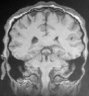 [T*]
[T*]
|
| ||||||||||||||||||||||||||||||||||||||||||||||||||||||||||||||||||||||||||||||||||||||||||||||||
The result of the registration is evaluated by the mean Euclidean
distance between the synthetic transformation T* used to deform the
image and the transformation T found by the registration
algorithm:



 |
[3D MRI 1]
 [3D MRI 2]
|
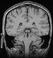
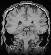
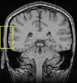
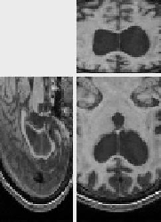
The original images were previously rigidly registered with the robust algorithm of [20]. One of the original image does not show the top of the head, which explains why a part of the skull is missing at the bottom of the rigidly registered image 5(a).
We used a Gauss-Newton-like gradient descent with the SLCC formula to register the images, and a Gaussian with a standard deviation of 1.8 to smooth the transformation.
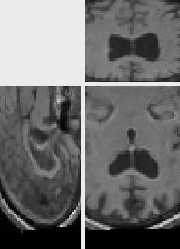
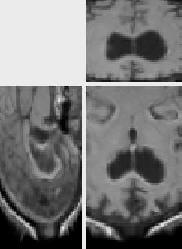
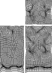
The results presented in Fig. 6 have been obtained in 103 seconds on a 450MHz Pentium II. They show a good match of the structures, as well as a smooth transformation, with deformations localized near the ventricles and the missing part of the skull. This later movement is due to the lack of specific treatment of occlusions in our algorithm. Results using the LCC formula are almost the same, but run in 127 seconds.
A remarkable fact is that an isovalue of the Jacobian of the recovered
transformation almost perfectly segments the ventricles which have
grown between both acquisitions. The dilatation ratio recovered by the
transformation is the same for big structures as well as small
structures.
We have also registered these images using the SSD criterion, and a
uniform correction of the bias and contrast change, i.e. we have set
![]() and registered
I' and J, I being image 5(a). The registration ran in
64 seconds. The results are poor: this is due to the fact that the
uniform intensity correction is not efficient. For example, the
background intensity is 0 in J but -9 in I', which explains
the problems near the skull. The intensity value of white matter is
also underestimated (100 instead of 120). The uniform intensity
correction does not work because the histogram is altered by changes
(the skull occlusion and mainly the growth of the ventricles) other
than the bias and contrast change.
and registered
I' and J, I being image 5(a). The registration ran in
64 seconds. The results are poor: this is due to the fact that the
uniform intensity correction is not efficient. For example, the
background intensity is 0 in J but -9 in I', which explains
the problems near the skull. The intensity value of white matter is
also underestimated (100 instead of 120). The uniform intensity
correction does not work because the histogram is altered by changes
(the skull occlusion and mainly the growth of the ventricles) other
than the bias and contrast change.
 |
In this paper, we showed how to use the derivatives of the sum of local correlation coefficients (LCC) everywhere in the image to drive a non-rigid registration algorithm. This is computationally feasible thanks to the Gaussian window because we can compute the derivatives very efficiently using separable Gaussian filters. We also compared two gradient descent techniques, an adaptation of the Gauss-Newton method and a linear search, to optimize this non quadratic criterion.
We found that the LCC and its approximation SLCC are almost as accurate as the SSD on images without bias. They work almost as well with biased images, where the SSD fails, showing the robustness of this criterion with respect to non-uniform bias. The LCC and the SLCC methods demonstrate equivalent accuracies, but SLCC is faster than LCC: they were respectively 1.75 and 2.50 times slower than the SSD in our experiments.
A few points still need to be investigated to fully control and automate the algorithm. Firstly, we have to study the impact of the boundary conditions of the filters on the computations of the similarity measure and the gradient. The spread of the Gaussian window used to compute the local statistics could be chosen automatically. Last but not least, we should study and compare the behavior of our technique using a minimization of the sum of the similarity and the smoothing energies.
We believe that numerous non-rigid registration algorithms that use dense (i.e., at each voxel) forces to guide the registration could be extended from the SSD to the LCC criterion using the approach presented here. Moreover, even if we presented the formulas and the experiments with the sum of local correlation coefficients, the method is intrinsically generic and could be applied to many other local criterions, the only limitation being the ability to compute the derivative of the criterion.