Purpose

espace enables to visualize various workspaces for a 3-RPR planar parallel robot, and to plan motion for this kind of robot, insuring that the trajectory always lie inside the robot workspace.

Let C define a given point on the moving platform. These workspaces are:

constant orientation workspace. This workspace is defined as the region which can be reached by C when the orientation of the moving platform is kept constant.
maximal workspace, which is defined as the region which can be reached by C with at least one orientation.
inclusive workspace, i.e. the region which can be attained by point C with at least one orientation in a given range.
total orientation workspace, i.e., the region which can be reached by point C with every orientation of the platform in a given range.
dextrous workspace, which is defined as the region which can be reached by point C with any orientation of the platform.

Availability

Free source codes are available under Free Software Society conventions through anonymous ftp (download here for Sun, download here for Linux).

This software is provided "as is" without warranty of any kind. In no event shall INRIA be liable for any loss of profits, loss of business, loss of use or data, interruption of business, or for indirect, special, incidental, or consequential damages of any kind, arising from any error in this software.

Implementation feature

Window system: X
Type: sources
Language: C
OS:Solaris,linux
Total number of lines: around 27000
Size of the executable: 3.5 Mo (Solaris),2 Mo (linux)
Output: display, files, graphic output in xjpdraw format

User's manual

espace user's manual Version 0.1
July 26, 1995

J-P. Merlet
INRIA Sophia-Antipolis
France
E-mail: Jean-Pierre.Merlet@inria.fr

Introduction

espace enables to visualize various workspaces for a 3-RPR planar parallel robot, and to plan motion for this kind of robot, insuring that the trajectory always lie inside the robot workspace. It is an implementation of the algorithms described in [1].

Let C define a given point on the moving platform. These workspaces are:

constant orientation workspace. This workspace is defined as the region which can be reached by C when the orientation of the moving platform is kept constant.
maximal workspace, which is defined as the region which can be reached by C with at least one orientation.
inclusive workspace, i.e. the region which can be attained by point C with at least one orientation in a given range.
total orientation workspace, i.e., the region which can be reached by point C with every orientation of the platform in a given range.
dextrous workspace, which is defined as the region which can be reached by point C with any orientation of the platform.

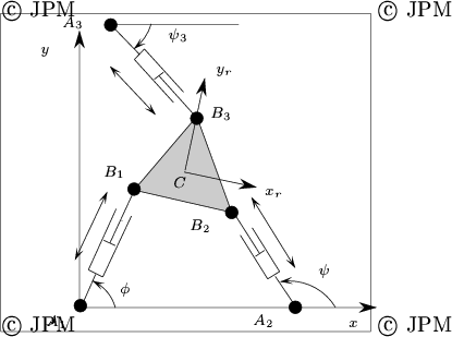
The 3-RPR robot is constituted of a moving platform connected to the ground through three revolute-prismatic-revolute kinematic chains (figure 1).

**Figure 1:** The 3-RPR robot
$\begin{figure} \begin{center} \ifx\cs\tempdima \newdimen \tempdima\fi \ifx\cs\te... ...si_3$ } \end{picture}\setlength{\unitlength}{1cm} \par\end{center} \end{figure}$

Mechanism description

The mechanism is defined via two structures:

struct quatre_barres
{

        float p;
        float r;
        float s;
        float c;
        short int coupler; /* 1 if the coupler exists */
        float a;
        float b;
        float sgamma; /*sine and cosine of gamma */
        float cgamma;
};
struct cinq_barres
{
        struct quatre_barres sous_4barres;
        float or[2];
        float r3;
}

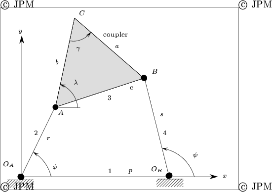
Indeed the 3-RPR robot is constituted of a four bar mechanism whose elements are defined in figure 2, with an additional link whose attachment point to the ground A3 has coordinates stored in or and whose length is r3.

**Figure 2:** A four bar mechanism
$\begin{figure} \begin{center} \ifx\cs\tempdima \newdimen \tempdima\fi \ifx\cs\te... ...){$B$ } \end{picture}\setlength{\unitlength}{1cm} \par\end{center} \end{figure}$

Therefore the three length of the chains are r, s, r3. To use this program you need to define the structure of the robot in a file with the following syntax A file defining a 3-RPR mechanism has the following syntax:

5-barres
p
r
s
c
1
a
b
sgamma
cgamma
or[0]
or[1]
r3

The value of the leg lengths defined in this file are only used to display the robot in one one of its configuration when running the program. To specify the minimal and maximal values of the leg lengths you need to create another file which contain these values. For example the file:

specify that the minimum value for r is 2, its maximal value 8, then you got the value for s and r3.

To run the program use the command:

 
espace [mechanism file] [extremal lengths file]

The mechanism will be displayed in a nominal position. By definition the vertices of the moving platform are called B1, B2, B3 which are connected to the leg of length r, s, r3.

The `Maximal Workspace(B3)` button

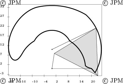
This buttons enable to compute the maximal workspace for the reference point B3. After having clicked in this button you should see the drawing of the maximal workspace (this may take some time, up to 30s for very complex cases). The boundary of the maximal workspace is displayed in green. Inside the region you may see also various curves in different colors. These regions may define sub-maximal workspace, i.e. maximal workspace according to an initial assembly configuration. To check that put the cursor in the screen, on top of the display you will see the current location in the reference frame of the robot (whose center is located at A1), and the possible orientation of the robot for the current location (note that the orientation is defined as the angle between Ox and B3B1). The possible orientation is a list of intervals. You may notice that when crossing a curve in the maximal workspace, the number of possible orientations intervals will vary.

The `Save Maximal Workspace` button

This button is used after having computed the maximal workspace and enable to save a description of the workspace in a file. This description has no interest for the user's but will be used by espace when planning a trajectory. If a file describing the maximal workspace has been saved the computation time for planning a trajectory will be drastically reduced.

The `Maximal Workspace(B123)` button

This button is used to display the three maximal workspaces when the reference point is defined as B1, B2, B3.

The `Orientation workspace` button

This button enable to compute the workspace of B3 when the orientation of the moving platform is constant. Give a value for the orientation angle (the rotation angle is the angle between Ox and B1B3) and press Return.

The `Maximal Workspace(IOW)` button

This button enables to compute the inclusive orientation workspace for B3, i.e. all the position of B3 such that the possible orientations of the robot has an intersection with an orientation range. For example if the range you have defined is [300, 310] and the possible orientation of the robot is [270, 305] for a given position of B3, then this position is inside the IOW. Give the range as two angles in degree, followed by a return.

The `Maximal Workspace(TOW)` button

This button enables to compute the total orientation workspace for B3, i.e. all the position of B3 such that the possible orientations of the robot include an orientation range. For example if the range you have defined is [300, 310] and the possible orientation of the robot is [270, 315] for a given position of B3, then this position is inside the TOW. Give the range as two angles in degree, followed by a return. Note that giving an orientation range of [0,360] enables to compute the location of B3 such that every orientation is possible, i.e. the TOW is the dextrous workspace of the robot.

The `Configuration` button

The robot will be displayed if you give the position of B3 (two coordinates) and the orientation (in degree). The color of the legs will be be red if the link length is outside the allowed range and blue otherwise.

The `Motion planning` button

When clicking in this button you will be able to plan motion for the robot. First the program will compute and display the maximal workspace of the robot. Note that if you have previously computed this workspace and saved it, then the motion planner will directly use the file. Then an auxiliary computation is done (which is computing a skeleton as described in [1]).

Then a new window will appear where you can indicate a start and a goal configurations. First introduce the start configuration, followed by a Return, then the goal configuration, followed by a Return. The planner will then try to compute a trajectory: by default the planner look for the shortest trajectory. You can change this by clicking in the Priority button: if the priority is length the planner will look for the shortest path, if the priority is orientation the planner will try to preserve the orientation (for example if the start and goal configuration have the same orientation it will look for a trajectory on which the orientation remains the same). If the priority is circular the planner will look for a circular trajectory if the start and goal have same orientation, in which the constant orientation workspace will be displayed. You can also define a desired trajectory together with a priority in a file in which you define the three coordinates of the start points, the three coordinates of the end point and then a keyword for defining the priority, either length or orientation. Note that when a trajectory is displayed the leg lengths are also displayed on top of the screen.

The Read Trajectory File enables to display a pre-computed trajectory. The Redraw button enables to redraw the trajectory. By using the Slowness button you can adjust the velocity of the robot, the greater the value, the slowest the velocity. After having computed a trajectory you can save it using the Save trajectory button.

`Zoom, Origin` buttons

These buttons may be used to modify the location of point OA on the screen or to zoom the drawing. To zoom give a scale factor followed by a Return in the Zoom window. A number lower than 1 will enable to reduce the size of the display. To indicate a new position of OA give its new screen coordinates in the window, followed by a Return.

Miscellaneous buttons

The Clear button erase the screen, the Time button indicates the computation time for the last action, the Time(s) button will display the computation time of the skeleton.

The Debug button is used to debug this program. Although not very useful for a user it can be used to display the geometrical element which appear during the computation of the workspaces: for example the sextics, circles will be displayed.

`Jpdraw` button

xjpdraw is a drawing editor which accept external inputs and is available via anonymous ftp. This button is used to save in xjpdraw format what is currently on the screen.

if you have computed the maximal workspace for B3 the name of the generated files are: espace_maxi.jpd (with only the border of the maximal workspace) and espace_max_entier.jpd which contains the border but also the internal arc.
if you have computed the three maximal workspaces the name of the file is espace_max123.jpd
if you have computed the constant orientation workspace the name of the file is espace_orientation_[value].jpd, where value is the closest integer to the orientation angle.
if you have computed the IOW the name of the file will be espace_maxi_angle_[value1]_[value2].jpd where value1, value are the closest integers to the angles of the range
if you have computed the TOW the name of the file will be espace_teta_angle_[value1]_[value2].jpd where value1, value are the closest integers to the angles of the range
if you have displayed a robot the file name will be robot_configuration.jpd

Using the graphical outputs

To use one of the graphical output files, e.g. pos.jpd use xjpdraw with the command line:

 
xjpdraw -X 6 -Y 6 -F pos.jpd

where the numbers following the X and Y argument are the width and height of the box which will contain the output data.

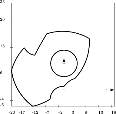
Here are some examples of drawing generated.

**Figure 3:** Example of maximal workspace
$\begin{figure} \begin{center} \ifx\cs\tempdima \newdimen \tempdima\fi \ifx\cs\te... ...tsize \end{picture}\setlength{\unitlength}{1cm} \par\end{center}\end{figure}$

**Figure 4:** Example of IOW
$\begin{figure} \begin{center} \ifx\cs\tempdima \newdimen \tempdima\fi \ifx\cs\te... ...2.50){33} \end{picture}\setlength{\unitlength}{1cm} \end{center}\end{figure}$

**Figure 5:** Example of TOW
$\begin{figure} \begin{center} \ifx\cs\tempdima \newdimen \tempdima\fi \ifx\cs\te... ...jpdrawx}} \end{picture}\setlength{\unitlength}{1cm} \end{center}\end{figure}$

Using the command language

You can also use a command language for controlling the behavior of the program. To do that you write a file and run the program with the command

 
espace -C [command file]

If instead C you use I then no window will appear, the program will just execute the command file without displaying any result on the screen. You will have a similar behavior if you put at the start of your command file the keyword hidden.

One of the first instruction should be the definition of your robot with:

 
robot "robot file name"

Then you define the minimal and maximal leg length with:

 
length "5 20 5 25 6 30"

where 5, 20 define the length range for link 1 and so on. When this instruction is encountered and a robot has been defined the program will compute and display the maximal workspace.

This language has variables whose names are %0, %1 and so on and vectors whose names are %v0, %v1 and so on. In this language you have loop instructions (while, for), conditional instructions and you can perform operation on the variable, see the xjpdraw manual for more details.

You can compute the possible orientation angles for a position as:

 
%v0[0]=1
%v0[1]=2
%1= angle_limite ( %v0 , %v1 , %v2 )

%v0 define the coordinate of the position and %1 will contain the number of orientation intervals, the start of the intervals being put in %v2.

You can define an orientation with:

 
orientation= %10

You can test if a point is inside the workspace with

 
%5= point_in_space ( 10, 20, 300 )

where the three number define the position and orientation.

You can compute a TOW with:

 
variable= espace_orientation_total variable variable

where the two last variables define the orientation angle range in degree. You can compute a IOW with:

 
variable= espace_orientation_inclusive variable variable

where the two last variables define the orientation angle range in degree. You can compute a constant orientation workspace with:

 
variable= espace_orientation variable

where the last variables define the orientation angle in degree. In all these cases the first variable contains the number of zone of the computed workspace.

You can display information on the screen during the execution of the program with:

 
info " string to be printed"

For the motion planning you define the start and goal configuration with:

 
start u1 u2 u3
goal v1 v2 v3

where the u's and v's may be either numbers or variables and define the position and orientation of the robot.

You can set the priority with priority_length, priority_orientation.

You can look for a trajectory with:

 
%1= mode find_trajectory

In return the variable will have the value 1 if a trajectory has been found.

The current result of the computation could be saved in xjpdraw format with:

 
save "file name".%1 "auxiliary file name".%2

The result will be in general save in the file

 
file name".%1

but if two files are to be saved the second name will be used. To quit the program use quit.

Bibliography

1: Merlet J-P. and Mouly N.
Espaces de travail et planification de trajectoire des robots parallèles plans.
Research Report 2291, INRIA, 1994
GET IT!ftp://ftp-sop.inria.fr:/pub/rapports/.

La page Présentation de COPRIN

La page "Présentation" de l'INRIA

Jean-Pierre Merlet