Univariate polynomials and series

The basic types to use for computing with polynomials and series are DenseUnivariatePolynomial and DenseUnivariateTaylorSeries respectively. Both types are univariate but can be nested if needed to produce dense multivariate polynomials and series with a fixed number of variables. When the number of variables is too large for a dense representation, you can also use SparseUnivariatePolynomial but be aware that for univariate or bivariate use, its arithmetic is much less efficient than the one of DenseUnivariatePolynomial.

As for matrices, the type of the coefficients of polynomials or series does not need to be a Ring, it can be an ArithmeticType instead. This allows types that do not have a full equality such as SingleFloat to be used as coefficients, but some polynomial functionalities are only available when the coefficient type is a Ring or something stronger. The polynomial and series types take a Symbol as second argument. That symbol is used only for output when converting the polynomial or series to an ExpressionTree, so it is not necessary to give one when you use polynomials or series inside a calculation. If you insist on naming the variable, use $-$ with any string as argument to create a symbol. For example, DenseUnivariatePolynomial(Integer) and SparseUnivariatePolynomial(Fraction Integer, -"x") are both valid polynomial types. Whether you give a name for a variable or not, you can override that choice using apply with a Symbol or ExpressionTree as argument. For example, if $p$ is a polynomial or series, stdout(p, -"z") writes $p$ to stdout using ``z'' as variable name, and p(extree leaf(-"y")) returns the ExpressionTree corresponding to $p$ with ``y'' as variable name.

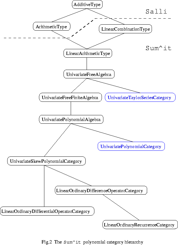
To write generic code for manipulating polynomials or series use a type parameter usually of category UnivariatePolynomialCategory or UnivariateTaylorSeriesCategory respectively. Because polynomials, skew-polynomials and series share many common operations, $\Sigma{}^{{\rm it}}$ provides in fact a complete category hierarchy for them, shown in Figure 2.

Those categories make it possible to write functions that work for polynomials, skew-polynomials, series or any combination of them. UnivariatePolynomialCategory$(R)$ is the category for types whose elements are usual polynomials of the form $\sum_n r_n x^n$ with finite support. While $R$ is not assumed to be commutative, the generator $x$ is assumed to commute with coefficients in $R$, i.e. $rx = xr$. Similarly, UnivariateTaylorSeriesCategory$(R)$ is the category for types whose elements are series of the form $\sum_n r_n x^n$. Here also, $R$ is not assumed to be commutative, but the generator $x$ commutes with coefficients in $R$. Those two categories are shown in blue in Figure 2, as they are the only ones assuming that $x$ commutes with $R$. The more general category UnivariatePolynomialAlgebra$(R)$ is for types whose elements are sums of the form $\sum_n r_n x^n$ with finite support, but where $x$ does not necessarily commute with $R$. Polynomials and skew-polynomials are both in that category. Even more general, UnivariateFreeFiniteAlgebra$(R)$ is for types whose elements are sums of the form $\sum_n r_n P_n$ with finite support, but where the family $P_n$ is not necessarily the power basis $x^n$. An example of such a type is UnivariateFactorialPolynomial for which $P_n = x(x-1)\dots(x-n+1)$. Finally, UnivariateFreeAlgebra$(R)$ is for types whose elements are potentially infinite sums of the form $\sum_n r_n P_n$. Code written at that level works for polynomials, series and skew-polynomials as well.

The elements of DenseUnivariateTaylorSeries are lazy series represented by their coefficient sequences, themselves of type Sequence. Those coefficient sequences are in turn represented as Stream from SALLI. Therefore, the usual way to write a function producing a series is to produce first its coefficient stream $s$, then call sequence on $s$ to produce the coefficient sequence, and finally call series on the coefficient sequence to produce the series. Since streams are lazy, constructing a series does not compute any of its coefficients until they are specifically requested by another operation. There are several ways to create streams, all documented in the SALLI reference manual, and you should become familiar with them before programming with series. For example, the following function takes constants $a_0$ and $c$ and produces the hypergeometric series $\sum_{n\ge 0} a_n x^n$ where $a_{n+1}/a_n = c$.

SeriesSample(R:CommutativeRing, Rx:UnivariateTaylorSeriesCategory R): with {
         hypergeometricSeries: (R, R) -> Rx;
} == add {
         hypergeometricSeries(a0:R, c:R):Rx == {
                import from Sequence F;
                zero? a0 => 0;
                -- the following creates the stream [a0, c a0, c^2 a0, ... ]
                coeffs:Stream R := orbit(a0, (x:R):R +-> c * x);
                series sequence coeffs;
         }
}