Computational Anatomy of the Brain
4. A Generative Model of Brain Populations Variability
4.1 A glimpse at the existing methods
To study the variability of the brain in populations, a first group of studies focused on voxel-based statistics [Hermoye et al. 2006, Giedd et al. 1999, Thompson et al. 2001]. In this case, one segments the brain into several regions of interest (grey matter, white matter, cerebro-spinal fluid, corpus callosum, thalamus) and one look at the evolution of the volume of such predefined regions of interest. In [Gogtay et al 2004], local density of grey matter is measured on each point of the cortex: this analysis at the voxel's level avoids the a priori definition of regions of interest that appears afterwards in the density maps. Some studies use DTI to perform longitudinal analysis like in [Barnea-Goraly et al., 2005] for example. However, the analysis is also mainly limited to the evolution of a single value: the fractional anisotropy calculated on anatomical landmarks. In every case, statistics on the evolution are performed on the basis of scatter plots. One computes linear or quadratic regression and then performs statistical tests (like Hotteling one) on the retrieved parameters to emphasize possible significant differences in the growth according to external features like gender, handedness, and ethnicity, or according to some developmental disorders like Childhood-onset schizophrenia or Williams syndrome. Eventually, like in [Gilmore et al, 2007], one measures anatomical differences across the population thanks to statistical tests performed on geometrical features such as cerebral asymmetry.
Another approach consists in deformation-based statistics ([Ashburner et al. 1998]) as initiated in [Chung et al. 2000a, Chung et al. 2000b, and Chung et al.2003] for temporal evolutions. In this approach the different acquisitions of the same subject are registered into the baseline leading to continuously time-dependent displacement field. Given this field for several subjects, one can fit a spatially varying linear deformation rate. Then, Hotelling's tests on the residuals determines the regions of brain where growth or atrophy is statistically significant. Notice that [Chung et al. 2003] synthesizes the evolution of surfaces by the evolution of geometrical invariants: area, volume and curvature. As far as we know, this is the first attempt to describe the anatomical variability in a more geometrical sense and to build a joint model that takes into account the variability both across a population and within a given subject's growth.
All these recent approaches enable to achieve some promising results. The specific role of the grey-matter evolution was highlighted and maturation of the brain was quantified. In particular, the process of myelination and its consequences was broadly discussed. Moreover, one emphasizes some major trends in the brain maturation and statistical tests enable to show significant differences between healthy and abnormal maturation. Such tests also reveal that external features like handedness have a significant impact on brain growth. However, the description of the brain maturation and the differences between different evolutions remain very simple. In most cases the whole geometry of the brain was summarized by the measure of its volume. Actually, the maturation issue was considered so far only as a problem of brain's volume growth. One would like to go one step further and describe the brain's anatomy more accurately. Looking at the volume evolution of sub-regions of the shape could not be satisfactory: we need continuous models of shapes and of their evolutions in order to provide a non-supervised geometric description of the difference between the evolution of two shapes. The central issue is actually to describe how the brain is growing, how anatomical structures like sulcal landmarks or cortical surfaces are developing through the time, how they differ one from another in a geometrical point of view.
A second feature that was not yet taken into account is the joint cross-sectional and longitudinal variability. Age is mainly considered as an absolute variable and data of different subjects are matched according to the age. The question of a possibly developmental delay or advance was not put so far.
Eventually, most of the models proposed in the literature are descriptive. The approaches based on statistical tests only state that there is a difference at the population level without providing a statistical model that explains the observed data. We believe that the conclusions would be more convincing if one could generate new observations according to a learnt statistical model. This would make obvious the variability captured by the model. Moreover such generative models could be also predictive: the classification parameters determined on a population in the learning phase can be turned into a classifiers on individual cases that could be used for diagnosis.
Our goal is therefore to define theoretical tools addressing the aforementioned limitations of the current work and to define statistical models that could be calibrated and tested on existing databases. Our strategy is to address the problem in two steps. First, we will define a generative statistical model for subjects of the same age. This model will able to capture a large range of geometrical variations, without reducing the shapes as a sets of arbitrary features. It will also combine deformation-based statistics and voxel-based statistics. Once this model will be defined and evaluated on real data, it will be extended in the next section to account for temporal evolutions. The resulting framework will therefore address both the geometrical and the temporal aspects.
4.2 A Generative Statistical Model at a Given Time-Point
In the medical imaging field, frameworks have been proposed to build atlases from databases of medical images [Joshi et al., 2004; Avants and Gee, 2004; Zollei et al., 2005] or from anatomical curves or surfaces [Glaunes and Joshi, 2006; Chui et al., 2004]. In both cases, the underlying idea is to estimate a "mean anatomy" (called also template or atlas in the literature), and then learn how this mean model deforms within a given population. We choose here to base our statistical estimation on a forward model, as pioneered in [Allassonniere et al., 2007; Ma et al., 2008]. This model appears to be particularly well suited for comparison between new data and the atlas, as explained in [Durrleman et al., 2008]. In this setting the observations are considered as a random perturbation of an unknown template, plus a residual perturbation.
The observations are given as discrete sampled objects. The template models an average continuous "ideal" biological material. The deformations of the template within the population capture the geometrical variability such as torque, stretching or shrinking effects. The residual perturbations is what remain once the geometrical variability has been discounted. It is measured by the differences between the observations and the deformed template (i.e. what cannot be captured by a regular deformation). It captures the variability in terms of "texture", which contains, for instance, change of topology, material creation or deletion, physical or numerical noise.
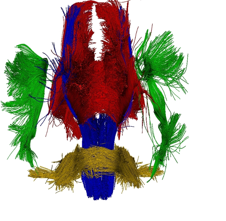
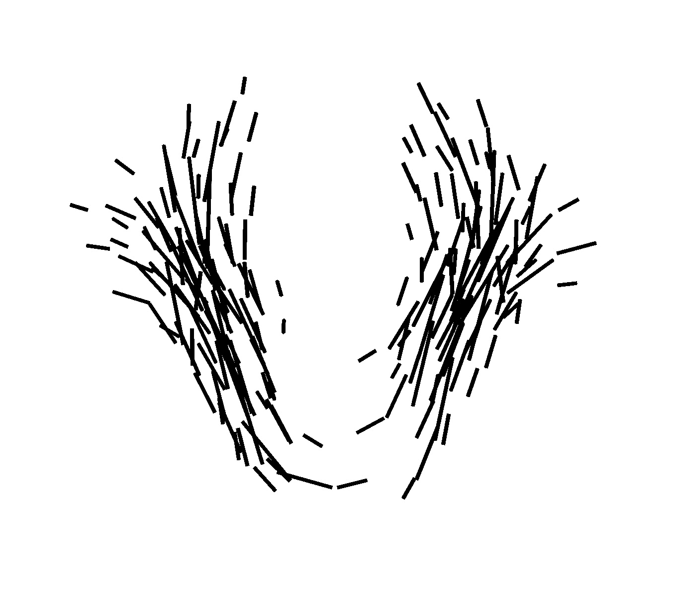
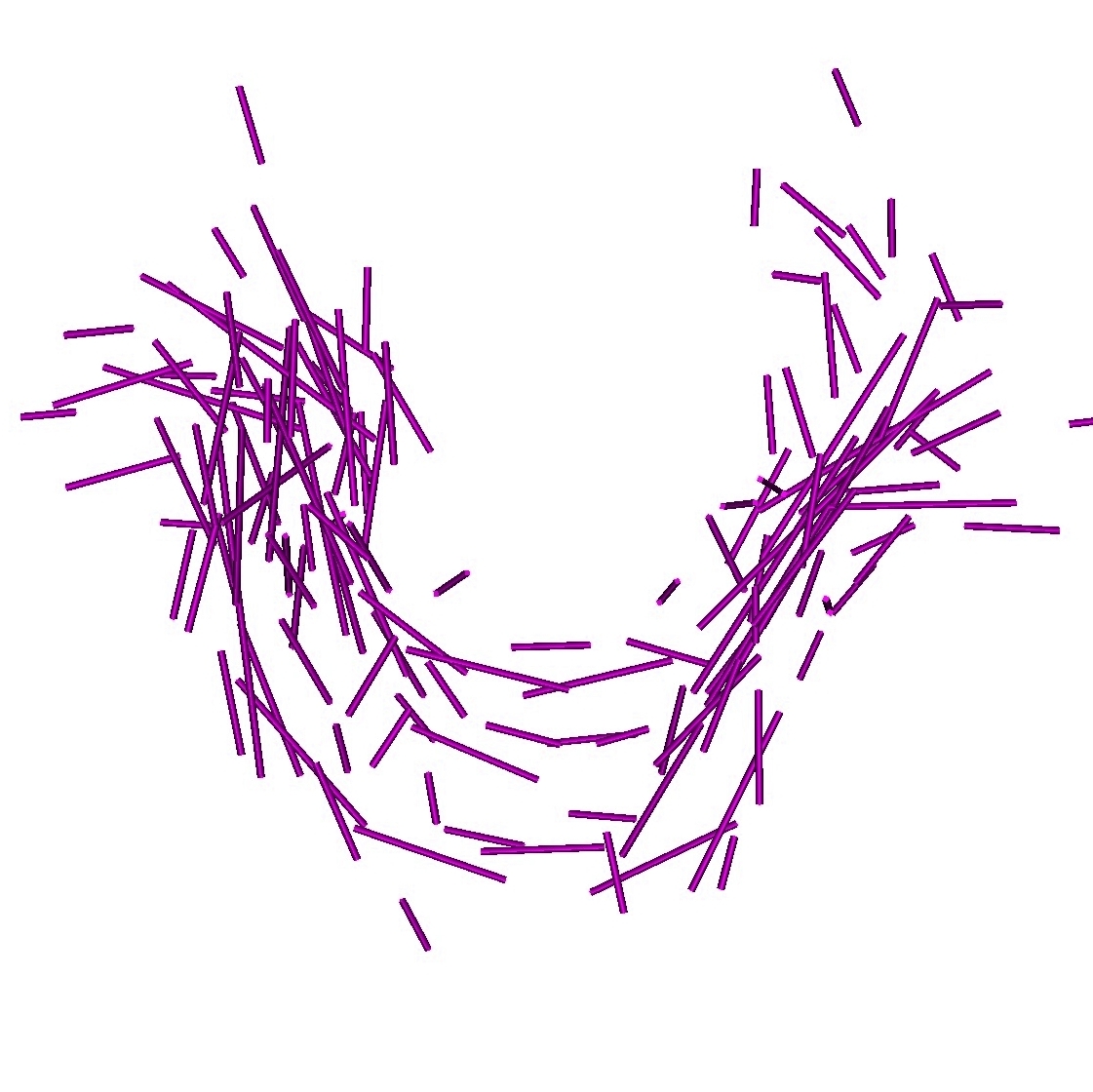
To estimate consistently the template, the deformations of the template in the population and the residual perturbation, we propose a Maximum A Posteriori approach. This approach takes advantage of the correspondence-less diffeomorphic approach detailed in Section 2 to deform the template to each subject's anatomy. Figure 1 present a template of white matter fiber bundles segmented in 6 subjects using MedINRIA.
 |
 |
 |
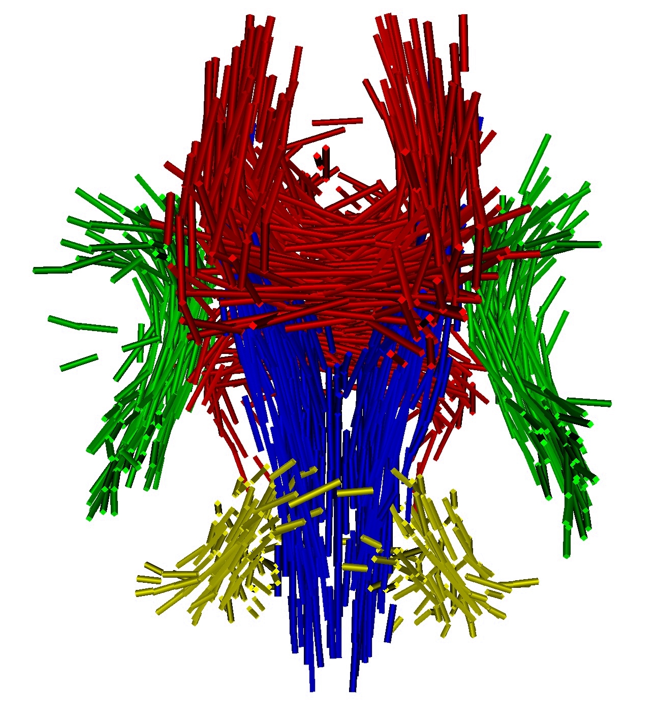
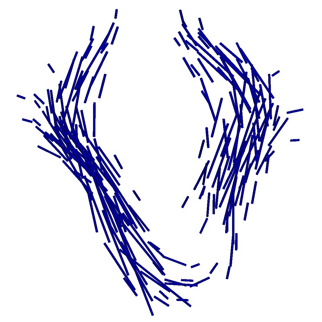
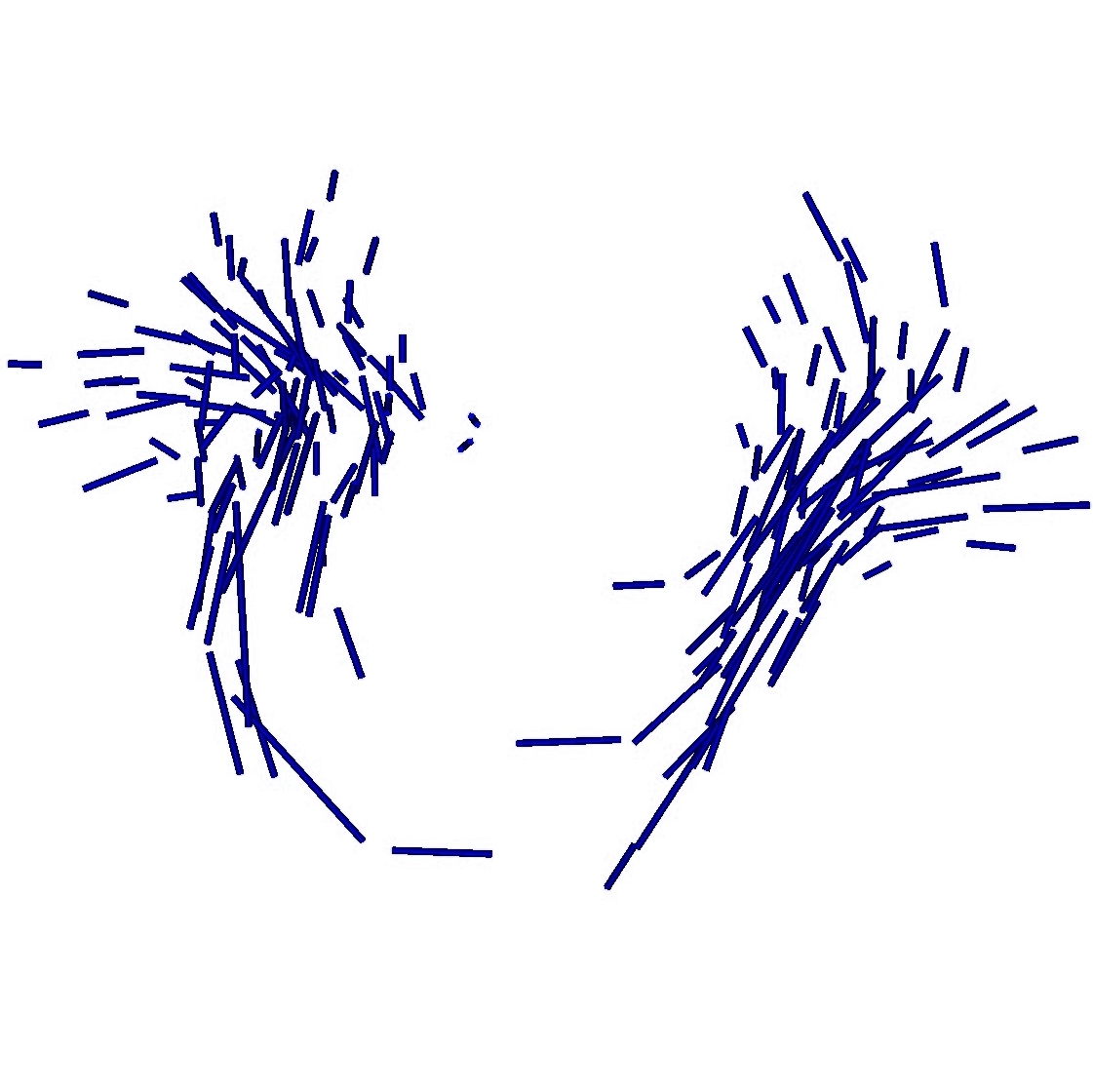
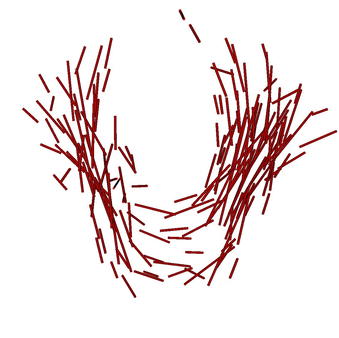
Once, the atlas is build, we can describe the variability within the population by analyzing (1) the geometrical variability captured by the deformations and (2) the variability in terms of texture captured by the residual perturbation. This is done by performing PCA on the deformations parameters and the residual currents respectively. This last PCA in the space of shapes is performed as shown in Section 3. Such a statistical analysis has been performed on our dataset of fiber bundles and results are shown in Fig. 2 and Fig. 3.
 |
 |
 |
 |
|
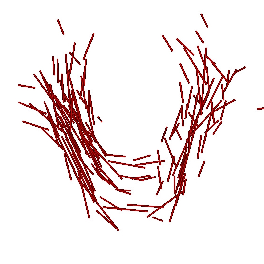 |
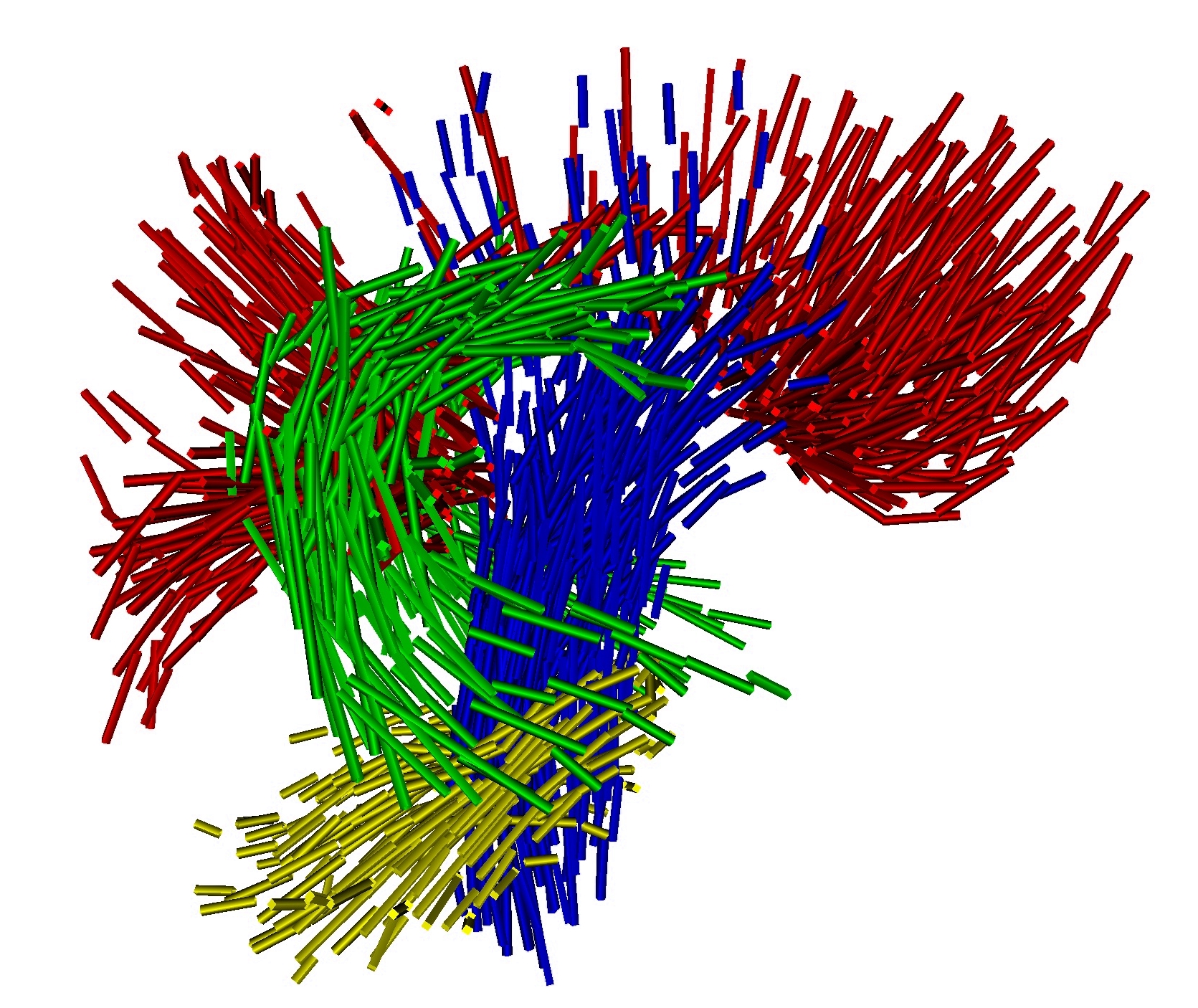
We can also use the atlas to generate new data according to the law we learn on data. We simulate an instance of the deformation, we deform the template according to this deformation and we add an instance of the residual to the deformed template. This is illustrated in Fig. 4.
|
|
 |
We can compute how likely a new observation could be according to our atlas. Given a new observation, we register the template to this data. This decomposes the variability between the observation and the template into a geometrical deformation and a residual perturbation. Then, we can measure the likelihood of the deformation's parameter and the residual current according to the Gaussian law we learnt on the parameter space and the space of currents. This could be used to classify new subjects according to their gender, handedness, pathologies, etc., as well as to detect abnormalities via deviations from the normal variability of the organs. One can also think of using the atlas to constraint the segmentation of the organs in images of new subjects.
4.3 References
- [Allassoniere et al., 2007] Allassonniere S., Amit Y., Trouvé A., Toward a coherent statistical framework for dense deformable template estimation. Journal of the Royal Statistical Society Series B 69 (1), p. 3-29, 2007
- [Ashburner et al., 1998] Ashburner J., Hutton C., Frackowiak R., Johnsrude I., Price C., Friston K., Identifying global anatomical differences: deformation-based morphometry, Human Brain Mapping 6, 1998
- [Avants and Gee, 2004] Avants B. and Gee J., Geodesic estimation for large deformation anatomical shape averaging and interpolation, Neuroimage 23, pp. 139-150, 2004
- [Barnea-Goraly et al., 2005] Barnea-Goraly N., Menon V., Eckert M., Tamm L., Bammer R., Karchemskiy A., Dant C.C., Reiss A.L., White Matter Development During Childhood and Adolescence: A Cross-sectional Diffusion Tensor Imaging Study, Cerebral Cortex, 2005
- [Carissa et al., 2007] Carissa J.C., Gerig G., Piven J., Diffusion Tensor Imaging: Application to the Study of the Developing Brain, Journal of the American Academy of Child and AdolescentPsychiatry, 2007
- [Chui et al., 2004] Chui H., Rangarajan A., Zhang J., Leonard C., Unsupervised learning of an atlas from unlabeled point-sets, IEEE Transactions on Pattern Analysis and Machine Intelligence 26 (2), pp. 160-172, 2004
- [Chung et al., 2000a] Chung M.K., Worsley K.J., Paus T., Cherif C., Collins D.L., Giedd J.N., Rapoport J.L. and Evans A.L., A Unified Approach to Deformation-Based Morphometry, NeuroImage, 2000
- [Chung et al., 2000b] Chung M.K., Worsley K.J., Paus T., Cherif C., Collins D.L., Rapoport J.L. and Evans A.L., Statistical Analysis of Local Volume Change, with an Application to Brain Growth, NeuroImage 2000
- [Chung et al., 2003] Chung M.K., Worsley K.J., Robbins S., Paus T., Taylor J., Giedd J.N., Rapoport J.L. and Evans A.L., Deformation-Based Surface Morphometry Applied to Gray Matter Deformation, NeuroImage:18(2), 2003
- [Durrleman et al., 2007] Durrleman S., Pennec X., Trouvé A., Ayache N., Measuring Brain Variability via Sulcal Lines Registration: A Diffeomorphic Approach, Proc. Medical Image Computing and Computer Assisted Intervention (MICCAI), LNCS 4791, pp. 675-682, 2007
- [Durrleman et al., 2008] Durrleman S., Pennec X., Trouvé A., Ayache N., A forward model to build unbiased atlases from curves and surfaces, Proc. of Mathematical fundations of Computational Anatomy, 2008
- [Evans et al, 2006] Evans A.L. and the Brain Development Cooperative Group, The NIH MRI study of normal brain development, NeuroImage 30(1):184-202, March 2006
- [Gerig et al, 2006] Gerig G., Joshi S., Fletcher T., Gorczowski K., Xu S., Pizer S.M. and Styner M. Statistics of population of images and its embedded objects: driving applications in neuroimaging. In Proc. of IEEE ISBI, pp1120-1123, April 2006.
- [Giedd et al., 1999] Giedd J.N., Blumenthal J., Jeffries N.O., Rajapakse J.C., Vaituzis C., Liu H., Berry Y.C., Tobin M., Nelson J., Castellanos X., Development of the human corpus callosum during chilhood and adolescence: a longitudinal MRI study, Prog. Neuro-Psychopharmacol. & Biol. Psychit. 23, 1999
- [Gilmore et al., 2007] Gilmore J., Lin W., Prastawa M., Looney C., Vetsa Y.S., Evans D., Smith J., Hamer R., Lieberman J., Knickmeyer R., Guido G., Regional Gray Matter Growth, Sexual Dimorphism and Cerebral Asymmetry in the Neonatal Brain, The Journal of Neuroscience 27, 2007
- [Glaunès and Joshi, 2006] Glaunès J. and Joshi S., Template estimation from unlabeled point set data and surfaces for Computational Anatomy, Proc. of Mathematical Foundations of Computational Anatomy, 2006
- [Gogtay et al., 2004] Gogtay N., Giedd J.N., Lusk L., Hayashi K., Greenstein D., Vaituzis C., Nugent III T.F., Herman D.H., Clasen L.S, Toga A., Rapoport J.L., Thompson P.M., Dynamic mapping of human cortical development during childhood through early childhood, P.N.A.S., 2004
- [Hazlett et al, 2005] Hazlett, H.C., Poe, M., gerig, G., Gimpel Smith R.,Provenzale J., Ross Å, Gilmore J.H. and Piven J. Magnetic resonnance imaging and head circumference study of brain size in autism. In The Archives of General Psychiatry, vol. 62, pp.1366-1376, December 2005.
- [Hermoye et al., 2006] Hermoye L., Saint-Martin C., Cosnard G., Lee, S.-K., Kim J., Nasogne M.-C., Menten R., Clapuyt P., Donohue P.K., Hua K., Wakana S., Jiang H., van Zijl P.C.M., Mori S., Pediatric diffusion tensor imaging: Normal database and observation of the white matter maturation in early childhood, NeuroImage 29, 2006
- [Joshi et al., 2004] Joshi S., Davis B., Jomier M., Gerig G., Unbiased diffeomorphic atlas construction for Computational Anatomy, Neuroimage 23, pp. 151-160, 2004
- [Ma et al, 2008] Ma J., Miller M., Trouvé A., Younes L., Bayesian template estimation in Computational Anatomy, Neuroimage 42 (1), pp. 252-261, 2008
- [Paus et al., 2001] Paus T., Collins D.L., Evans A.C., Leonard G., Pike B., Zijdenbos A., Maturation of white matter in the human brain: A review of magnetic resonance studies, Brain Research Bulletin, 54, 2001
- [Prastawa et al., 2005] Prastawa M., Gilmore J.H., Lin W., Gerig G., Automatic segmentation of MR images of the developing newborn brain, Medical Image Analysis: 9, 2005
- [Thompson et al., 2001] Thompson P.M., Vidal C., Giedd J.N., Gochman P., Blumenthal J., Nicolson R., Toga A.W., Rappoport J.L., Mapping adolescent brain change reveals dynamic wave of accelerated gray matter loss in very early-onset schizophrenia, P.N.A.S. 98, 2001
- [Vaillant and Glaunes, 2005] Vaillant M., Glaunes J., Surface Matching via Currents, Proc. of Information Processing in Medical Imaging, 2005
- [Zollei et al., 2005] Zollei L., Learned-Miller E., Grimson E., Wells W., Efficient population registration of data, Proc. of Computer Vision for Biomedical Image Applications, LNCS 3765, pp. 291-301, 2005