|
Border bases
|
Border basis algorithms provide an efficient way to compute the ring
structure of  , which is represented by
 a vector space of polynomials, which
corresponds to the normal form of the elements of the equivalent
classes of
a vector space of polynomials, which
corresponds to the normal form of the elements of the equivalent
classes of  ,
,
 a projection onto
  ,
with kernel
,
with kernel  , which computes the normal
form of the elements of
, which computes the normal
form of the elements of  modulo the ideal
.
modulo the ideal
.
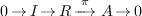
This means that we have the exact sequence:
with  . Normal form algorithms compute an
explicit basis (usually a monomial set) of and
an effective projection (usually a reduction process).
. Normal form algorithms compute an
explicit basis (usually a monomial set) of and
an effective projection (usually a reduction process).
Celebrate Gröbner basis computation provides such a normal form. Border basis is also a normal form algorithm, which generalizes Gröbner basis.
Assume that is graded by a ordered additive
monoïd that we denote  (for instance
  if we use the classical notion of degree): there
exists a degree function
if we use the classical notion of degree): there
exists a degree function  such that for any
 ,
,  .
.
The set of monomials of is denoted  . For
. For  , let
, let  be the vector space spanned by the set
  monomials of degree
  .
.
A border basis is defined with respect to a set  of monomials, connected to
  (if
(if  either
  or
or  and
and  such that
  ). Let
 and
and  . The computation
of a border basis goes through the construction of a family
. The computation
of a border basis goes through the construction of a family  of polynomials of the form
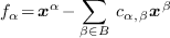
which are in  with only one term denoted
  in
in  . We illustrate it in
the following picture:
. We illustrate it in
the following picture:
The basis  corresponds to the light blue
region. The monomial in
corresponds to the light blue
region. The monomial in  are the thick points.
For
are the thick points.
For  , there is a polynomial
  with one monomial
  in
(e.g. the red thick point) and all the other monomials of its support
are in the light blue region . The polynomials
in
(e.g. the red thick point) and all the other monomials of its support
are in the light blue region . The polynomials
 can be used to rewrite all polynomials in as linear combinations of elements in modulo the ideal
  .
.
A family of polynomials of this form is called
a rewriting family. The family is graded if  for all
  . For
. For  , ,
, ,  is the
set of elements of
is the
set of elements of  of degree
  .
.
A rewriting family is said to be
complete in degree  if it is graded
and satisfies
if it is graded
and satisfies  ; that is, each monomial
  of degree at most is the
leading monomial of some (necessarily unique) .
of degree at most is the
leading monomial of some (necessarily unique) .
Given a rewriting family which is complete in
degree , we define recursively the projection
 on along in the following way:
  ,
,
if  , then
  ,
,
if  , then
 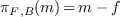 , where
 is the (unique) polynomial in for which
  ,
,
if  for some integer
  ,
write , where
,
write , where  and
and
 is the smallest possible variable index
for which such a decomposition exists, then
is the smallest possible variable index
for which such a decomposition exists, then  .
.
The map πF,B extends by linearity to a linear map from
 onto
onto  . By construction,
 and
and  for all
  .
.
The next theorem [?] shows that, under some
natural commutativity condition, the map
coincides with the linear projection from onto
along the vector space  :
:
 is connected to
  and let
  be a rewriting family for , complete in degree
  . Suppose
that, for all
. Suppose
that, for all  ,
,

(1)
Then coincides with the linear projection
of on along the
vector space  ; that is,
 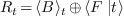 .
.
The commutation polynomials or  -polynomials are
the polynomials
-polynomials are
the polynomials  for ,
for ,
 such that
  or
or  . By this theorem, is a border
basis for in degree
iff all the -polynomials reduces to
. By this theorem, is a border
basis for in degree
iff all the -polynomials reduces to  , i.e. their image by is .
The border basis algorithm computes a rewriting family which satisfies the relation (?) for any
degree [?]. It proceeds
incrementally degree by degree with a candidate monomial set for the basis of and the
rewriting family for
at a given degree . At each degree, the
non-zero polynomials deduced from the relations (?) are
added to .
In the main loop of the algorithm, the following operations are performed:
prolongation: determine the new elements of in degree  and the elements
 of
of  which are in
 ;
;
matrix construction: compute the coefficient matrix  of with respect to
  ;
;
linear reduction: compute a (sparse)  decomposition of the matrix and update the
rewriting family ;
decomposition of the matrix and update the
rewriting family ;
commutation reduction: reduce the -polynomials
with respect to and update , and ;
This loop is iterated until a complete rewriting family for which satisfies (?) is obtained in the case
of a zero-dimensional ideal or until the Gotzmann regularity criterion
is satisfied [?]. The computation is controlled by a
choice function, which select “leading” monomials for the
construction of rewriting families.
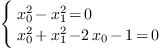
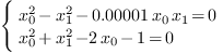
Let  . We consider the following polynomial
system:
. We consider the following polynomial
system:
The computed border basis for the monomial basis 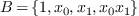 is
is
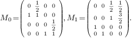
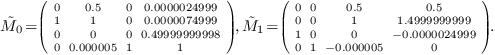
The matrices of multiplication by  ,
,
 in this basis are
The computation of a Gröbner basis for the degree reverse
lexicographic monomial ordering with  yields
the same basis and thus the same matrices of
multiplications by the variables , .
yields
the same basis and thus the same matrices of
multiplications by the variables , .
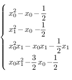
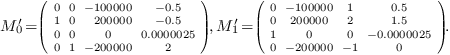
Consider now a small perturbation of the polynomial system:
The computed border basis is
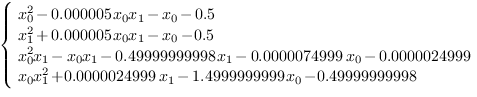
for the same monomial basis . The matrices of
multiplication by  in this basis are
These matrices are small perturbations of the multiplication matrices of the initial system. The order of the perturbation is the same as the order of the perturbation of the polynomial system.
If we compute a Gröbner basis for the degree reverse
lexicographic monomial ordering with  , we
obtain the basis
, we
obtain the basis 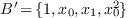 and the numerical
approximation (within
and the numerical
approximation (within  ) of the matrices of
multiplication by the variables in this basis
are
) of the matrices of
multiplication by the variables in this basis
are
We observe a great variation in the magnitude of the coefficients (of the order the inverse of the magitude of the perturbation in this example, but it could be worth!).
This illustrates the numerical stability of border basis computation and the instability of Gröbner basis computation against perturbations of the coefficients of the polynomial system.
[1] B. Mourrain and P. Trébuchet. Generalized normal forms and polynomials system solving. In M. Kauers, editor, ISSAC 2005: Proceedings of the ACM SIGSAM International Symposium on Symbolic and Algebraic Computation, pages 253–260. 2005.
[2] B. Mourrain and Ph. Trébuchet. Border basis representation of a general quotient algebra. In J. van der Hoeven, editor, ISSAC 2012, pages 265–272. Jul 2012.