|
Solving zero-dimensional equations
|
Let  be the ring of polynomials in the
variables
be the ring of polynomials in the
variables  with coefficients in
  . Let
. Let  be the equations to be
solved and
be the equations to be
solved and  the ideal of
  generated by these polynomials. The algebraic approach to solve the
equations
generated by these polynomials. The algebraic approach to solve the
equations  relies on the knowledge of
a basis  of
of  ,
,
a projection  with kernel
  , which computes the normal form of the elements of
modulo the ideal .
, which computes the normal form of the elements of
modulo the ideal .
Border basis computation (as well as Gröbner basis) provides
these two ingredients. They allow to compute the operators of
multiplication by an element  :
:

The matrix of the operator  in the basis
  is obtained by computing the normal forms
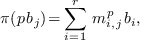
which yields the matrix 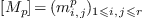 .
.
Let  be the dual of
  ,
that is the set of linear forms from to , which vanish on .
The transposed matrix is the matrix of the transposed operator
,
that is the set of linear forms from to , which vanish on .
The transposed matrix is the matrix of the transposed operator

in the dual basis of  .
.
The solution of a zero-dimensional systems relies on the analysis of the eigenspaces of these operators, provided by the following theorem [?, ?].
 with
with  . Let
. Let 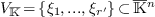 .
.
For any
The common eigenvectors of
, the eigenvalues of are 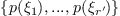 .
.
 are, up to
a scalar,
are, up to
a scalar, 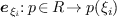 ,
, .
.
The evaluations are element of  , since by definition they vanish on all the polynomials
of (the points
, since by definition they vanish on all the polynomials
of (the points  are the
common roots of all the polynomials of ).
are the
common roots of all the polynomials of ).
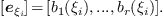
If is basis of , then
the coordinate vector of  in the dual basis of
is
in the dual basis of
is
By the previous theorem, we have

Therefore, the roots of the system can be recovered by computing the
matrices of multiplication by the variables in a basis of , then by computing the common
eigenvectors of the transposed matrices, deducing the evaluation at
the roots and thus the roots from these eigenvectors.
The resolution process consists in computing the roots from one or several operators of multiplication [?, ?].
The eigenspaces associated to the transposed operator  of multiplication by the variable
  in are computed. The first coordinates of the roots are
given by the eigenvalues of . If the
eigenspaces are one-dimensional the other coordinates are deduced.
Otherwise the transposed operator of multiplication by
in are computed. The first coordinates of the roots are
given by the eigenvalues of . If the
eigenspaces are one-dimensional the other coordinates are deduced.
Otherwise the transposed operator of multiplication by  restricted to these eigenspaces is computed as well as
its eigenspaces. It determines the second coordinates associated to a
given first coordinate. This process is repeated until all coordinates
of the roots are determined [?, ?].
restricted to these eigenspaces is computed as well as
its eigenspaces. It determines the second coordinates associated to a
given first coordinate. This process is repeated until all coordinates
of the roots are determined [?, ?].
For the linear algebra computation on dense matrices, a templated
version of
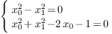
Let  . We consider the following polynomial
system:
. We consider the following polynomial
system:
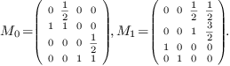
The computation of the border basis yields the monomial basis 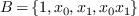 and the matrices of multiplication
by
and the matrices of multiplication
by  , :
, :
The computation of the eigenvectors of  gives:
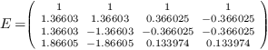
We have normalised the eigenvectors, so that their first coordinate is
 . As , these columns
correspond to the coordinate vectors of the evaluations
. As , these columns
correspond to the coordinate vectors of the evaluations

We deduce that the roots of system are

[1] E. Anderson, Z. Bai, C. Bischof, J. Demmel, J. Dongarra, J. Du Croz, A. Greenbaum, S. Hammarling an A. McKenney, S. Ostrouchov, and D. Sorensen. LAPACK Users' Guide. SIAM, Philadelphia, 1992. http://www.netlib.org/lapack/.
[2] M. Elkadi and B. Mourrain. Introduction à la résolution des systèmes d'équations algébriques, volume 59 of Mathématiques et Applications. Springer-Verlag, 2007.
[3] Stef Graillat and Philippe Trébuchet. A new algorithm for computing certified numerical approximations of the roots of a zero-dimensional system. In ISSAC2009, pages 167–173, July 2009.
[4] B. Mourrain. Computing isolated polynomial roots by matrix methods. J. of Symbolic Computation, Special Issue on Symbolic-Numeric Algebra for Polynomials, 26(6):715–738, Dec. 1998.
[5] P.M. Gianni R.M. Corless and B.M. Trager. A reordered schur factorization method for zero-dimensional polynomial systems with multiple roots. In Proceedings of the ACM International Symposium on Symbolic and Algebraic Computations, pages pp. 133–140, 1997.
[6] Philippe Trébuchet. A new certified numerical algorithm for solving polynomial systems. In SCAN2010, pages 1–8, July 2010.