Example 1

We will present first a very silly example of system in the three unknowns $x(1),x(2),x(3)$:

$$\begin{eqnarray*} && x(1)^2+2 x(1)+1=0 \\ && x(2)^2+2 x(2)+1=0 \\ && x(3)^2+2 x(3)+1=0 \end{eqnarray*}$$

Clearly this system has the unique solution (-1,-1,-1). We choose to define the TestDomain as the interval [-2,0] for all three unknowns. So we define a function which specify the TestDomain:

 
VOID SetTestDomain (INTERVAL_VECTOR & x)
{
  Resize (x, 3);
  x(1) = Hull (-2.0,0.0);
  x(2) = Hull (-2.0,0.0);
  x(3) = Hull (-2.0,0.0);
}

The we have to define the IntervalFunction:

 
INTERVAL_VECTOR IntervalTestFunction (int l1,int l2,INTERVAL_VECTOR & x)
// interval valued functions. The input are intervals for the
//variables and the output is intervals on the functions
//x are the input variables and xx the function intervals
{
INTERVAL_VECTOR xx(3);

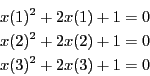
if(l1==1)  xx(1)=x(1)*(x(1)+2)+1;
if(l1<=2 && l2>=2)  xx(2)=x(2)*(x(2)+2)+1;
if(l2==3)  xx(3)=x(3)*(x(3)+2)+1;
  return xx;
}

This function returns the interval vector xx which will contain the value of the function from l1 to l2 for the box x. Note that the initial functions have been written in Horner form (or "nested" form) which may lead to a sharper estimation of the function intervals.

The main program may be written as:

 
INT main()
{
int Num; //number of solution
INTERVAL_MATRIX SolutionList(1,3);//the list of solutions
INTERVAL_VECTOR TestDomain;//the input intervals for the variable

//We set the value of the variable intervals
SetTestDomain (TestDomain);

//let's solve....
Num=Solve_General_Interval(3,3,IntervalTestFunction,TestDomain,
      MAX_FUNCTION_ORDER,50000,1,0.001,0.0,0.1,SolutionList,1);
//too much intervals have been created, this is a failure
if(Num== -1)cout << "The procedure has failed (too many iterations)"<<endl;
return 0;
}

This main program will stop as soon as one solution has been found. We set epsilonf to 0 and epsilon to 0.001 which mean that the maximal width of the interval solution will be lower than 0.001. The chosen order is the maximum equation ordering. The number of boxes should not be larger than 50000 and the distance between the distinct solutions must be greater than 0.1.

Running this program will provide the solution interval [-1.000977,-1] for all three variables and uses 71 boxes. The result will have been similar if we have chosen the maximum middle-point equation ordering.

On the other hand if we have epsilon to 0 and epsilonf to 0.001 the algorithm find the solution interval [-1.00048828125,-1] and use 78 boxes.

Now let's look at a more complete test program which enable to test the various options of the procedure.

 
INT main()
{
int Iterations;//maximal size of the storage
int Dimension,Dimension_Eq; // size of the system
int Num,i,j,order,precision,Stop;
// accuracy of the solution either on the function  or on the variable
double Accuracy,Accuracy_Variable,Diff_Sol; 
INTERVAL_MATRIX SolutionList(200,3);//the list of solutions
INTERVAL_VECTOR TestDomain;//the input intervals for the variable
INTERVAL_VECTOR F(3),P(3);

//We set the number of equations and unknowns and the value of the variable intervals
Dimension_Eq=Dimension=3;
SetTestDomain (TestDomain);

cerr << "Number of iteration = "; cin >> Iterations;
cerr << "Accuracy on Function = "; cin >> Accuracy;
cerr << "Accuracy on Variable = "; cin >> Accuracy_Variable;cerr << "Order (0,1)"; cin >>order;
cerr << "Stop at first solutions (0,1,2):";cin>>Stop_First_Sol;
cerr << "Separation between distincts solutions:";cin>> Diff_Sol;

//let's solve....
Num=Solve_General_Interval(Dimension,Dimension_Eq,IntervalTestFunction,TestDomain,order,Iterations,Stop,
      Accuracy_Variable,Accuracy,Diff_Sol,SolutionList,1);
//too much intervals have been created, this is a failure
if(Num== -1){cout<<"Procedure has failed (too many iterations)"<<endl;return -1;}
cout << Num << " solution(s)" << endl;

for(i=1;i<=Num;i++)
  {
    cout << "solution " << i <<endl;
    cout << "x(1)=" << SolutionList(i,1) << endl;
    cout << "x(2)=" << SolutionList(i,2) << endl;
    cout << "x(3)=" << SolutionList(i,3) << endl;
    cout << "Function value at this point" <<endl;
    for(j=1;j<=3;j++)F(j)=SolutionList(i,j);
    cout << IntervalTestFunction(1,Dimension_Eq,F) <<endl;
    cout << "Function value at middle interval" <<endl;
    for(j=1;j<=3;j++)P(j)=Mid(SolutionList(i,j));
    F=IntervalTestFunction(1,Dimension_Eq,P);
    for(j=1;j<=3;j++)cout << Sup(F(j)) << endl;
  }
  return 0;
}

This program is basically similar to the previous one except that it enable to define interactively the order, M, Stop, epsilon, epsilonf,Dist. Then it print the solution together with the function interval for the solution interval and the value of the functions at the middle point of the solution interval. Let's test the algorithm to find all he solution (Stop=0) with epsilonf=0 and epsilon=0.001. The algorithm will fail: indeed let's compute the maximal storage that we may need using the formula (2.1). We end up with the number $2^{6000}$ which is indeed a very large number.... But (2.1) is only an upper bound for the storage. For example if we have used epsilon=0.01 in the previous formula we will find that M=$2^{600}$ although the algorithm converge toward [-1,-0.992188] while using only 5816 boxes.

Although academic this system shows several properties of interval analysis. If we set epsilon=epsilonf=1e-6, which is the standard setting of ALIAS-Maple, the algorithm will run for a very long time before finding the solution of the system. Even using the 3B method, section 2.3.2 and the 2B method (section 2.17) the computation time, although improved, will still be very large. Now if we write the system as

$$\begin{eqnarray*} && (x(1)+1)^2=0 \\ && (x(2)+1)^2=0 \\ && (x(3)+1)^2=0 \end{eqnarray*}$$

the system will be solved with only 8 boxes, with 2 boxes if we use the 3B method and without any bisection if we use the 2B method. This shows clearly the importance of writing the equations in the most compact form.