where  is a domain of
  (in geometric modeling applications, usually
 ![$[0, 1]^2$](form_551.png) ) and
) and  are polynomials. The data structures for these rational maps is defined in
#include <synaps/shape/surface/MPDrationalSurface.h>
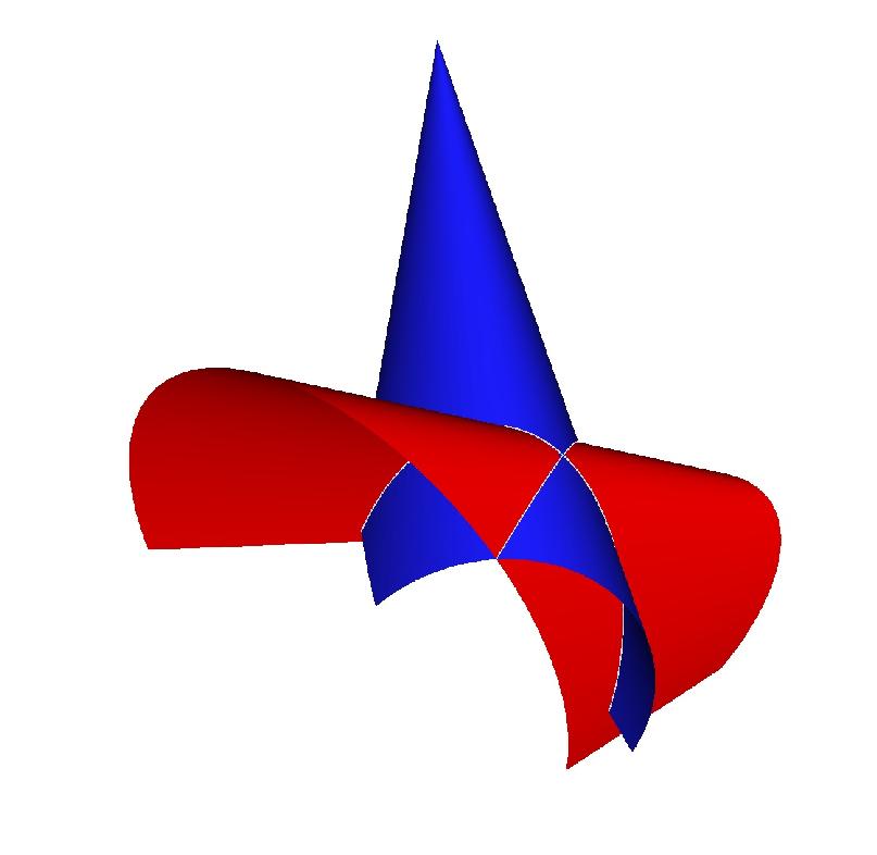
It can be defined easily from strings, as illustrated below:
![]()
![]()
# include <synaps/shape/interfaces/IRationalSurface.h>
# include <synaps/shape/surfaces/MPDRationalSurface.h>


int main(int argc, char** argv)
{
  using std::cout;
  using std::endl;
  MPolDseRationalSurface<double> s1, s2;

  s1.setEquations("s^2+t^2+1", "s-1+t^2", "s^2", "t^2", "s t");
  s1.setRange(-1, 1, -1, 1);

  s2.setEquations("s^2+t^2+1", "s*t-1", "t^2", "1-s^2", "s t");
  s2.setRange(-1, 1, -1, 1);

  cout<<s1<<endl;
  cout<<s2<<endl;

}
#include <synaps/base/io/axel.h>
This defines a axel ostream, which can be used as follows:
 axel::ostream vw("tmp.axl");
 vw<< s1;
 vw<<Color(25,25,225);
 vw<<s2;
 vw.view();
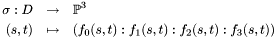
os<<Color(25,25,225); The color is describe in (red,green,blue) format with a integer number between 0 and 255. The surface s2 is printed, with this color. The view is displayed by the command vw.view(). It yields
![]()
![]()
# include <synaps/shape/interfaces/IRationalSurface.h>
# include <synaps/shape/surfaces/MPDRationalSurface.h>
# include <synaps/shape/surfaces/axel.h>


int main(int argc, char** argv)
{
  using std::cout;
  using std::endl;
  MPolDseRationalSurface<double> s1, s2;

  s1.setEquations("s^2+t^2+1", "s-1+t^2", "s^2", "t^2", "s t");
  s1.setRange(-1, 1, -1, 1);

  s2.setEquations("s^2+t^2+1", "s*t-1", "t^2", "1-s^2", "s t");
  s2.setRange(-1, 1, -1, 1);

  axel::ostream vw("tmp.axl");
  vw<<s1;
  vw<<Color(25,25,225);
  vw<<s2;
  vw.view();
}
 and
and  , given by the polynomials and
  , we want to compute their intersection points defined by the system:
![\[ (1) \left\{ \begin{array}{l} g_1 (u, v) f_0 (s, t) - f_1 (s, t) g_0 (u, v) = 0\\ g_2 (u, v) f_0 (s, t) - f_2 (s, t) g_0 (u, v) = 0\\ g_3 (u, v) f_0 (s, t) - f_3 (s, t) g_0 (u, v) = 0 \end{array} \right. \]](form_556.png)
This defines a curve in  which image by or in the intersection of the surfaces.
In order to visualise this intersection curve, we are going to fixe the values of ![$v \in [0, 1]$](form_558.png) and to solve the corresponding system in
and to solve the corresponding system in  and then compute the image of these points by .
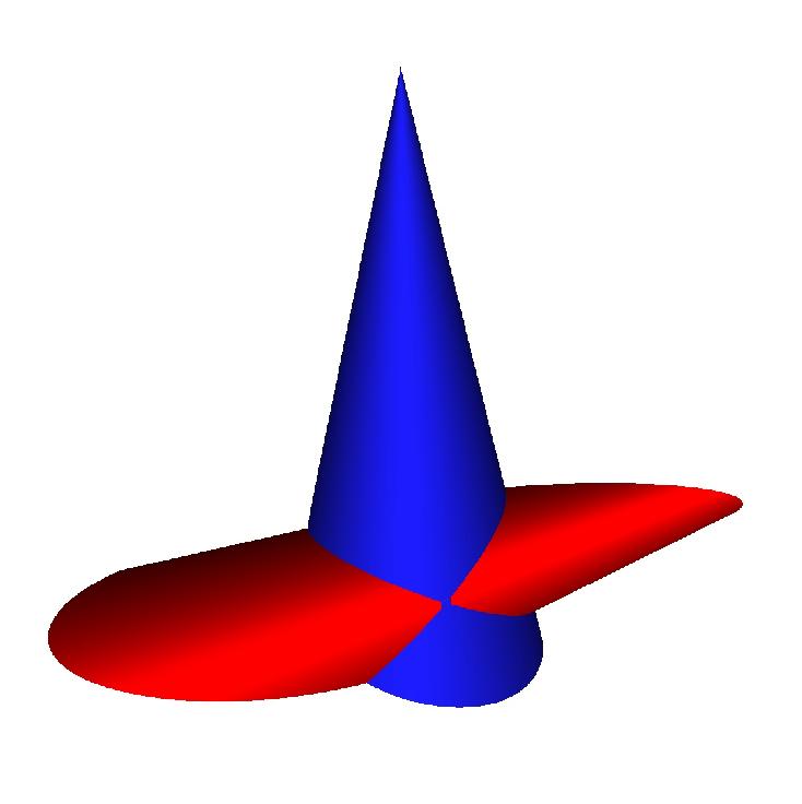
We are going to use the function intersect, which applies for anay paramteric surface. Its arguments are converted to pointers to IParametricSurface type. The result is of type IGLGood. It corresponds to a piecewise linear approximation of the result.
![]()
![]()
# include <synaps/shape/surfaces/MPDRationalSurface.h>
# include <synaps/shape/interfaces/IGLGood.h>
# include <synaps/shape/surfaces/axel.h>

int main(int argc, char** argv)
{
  using std::cout;
  using std::endl;
  MPolDseRationalSurface<double> s1, s2;

  s1.setEquations("s^2+t^2+1", "s-1+t^2", "s^2", "t^2", "s t");
  s1.setRange( -1, 1, -1, 1);

  s2.setEquations("s^2+t^2+1", "s*t-1", "t^2", "1-s^2", "s t");
  s2.setRange(  -1., 1., -1., 0.5);

  axel::ostream vw("tmp.axl");
  vw<<s1;
  vw<<Color(25,25,225);
  vw<<s2;
  IShape * r=intersect(&s1,&s2);
  IGLGood* g= r->mesh();
  vw << *g;
  vw.view();

}
Here is what we otain for the previous surfaces s1, s2: