| Modular numbers |
This document describes the use and implementation of the modulars within the numerix package.
1.General modulars and moduli
Moduli are implemented in modulus.hpp. An object of type modulus is declared as follows:
modulus<C,V> p;
V is an implementation variant. The default variant, named modulus_naive, is implemented in modulus_naive.hpp and supports a type C with an Euclidean division. More variants are described below. Modulars are implemented in modular.hpp. An object of type modular can be used as follows:
modular<modulus<C, V>, W> x, y, z;
modular<modulus<C, V>, W>::set_modulus (p);
x = y * z;
The variant W is used to define the storage of the
modulus. Default storage is modular_local
that allows the current modulus to be changed at any time. The default
modulus is  . For the integer
type the default variant is set to modulus_integer_naive,
so that modular integers can be used as follows:
. For the integer
type the default variant is set to modulus_integer_naive,
so that modular integers can be used as follows:
#include<numerix/integer.hpp>
#include<numerix/modular.hpp>
#include<numerix/modulus_integer_naive.hpp>

typedef modulus<integer> M;
M p (9973);
modular<M>::set_modulus (p);
modular<M> a (1), b (3);
c = a * b;
cout << c << "\n";
If the modulus is known to be fixed at compilation time then the following declaration is preferable for the sake of efficiency:
fixed_value <int, 3> w;
modulus<integer> p (w);
If the modulus is not intended to be changed and known at compilation time then the variant modular_fixed can be used.
2.Moduli for hardware integers
From now on  and
and  represent the quotient and the remainder in the long division of
  by
by  respectively. Throughout
this section C denotes a genuine integer C type. We
write
respectively. Throughout
this section C denotes a genuine integer C type. We
write  for the bit-size of C,
and for a modulus that fits in C.
for the bit-size of C,
and for a modulus that fits in C.
2.1.Naive implementation
The default variant, modulus_int_naive<m>,
is defined in modular_int.hpp. Each
modular product performs one product and one integer division. The
parameter m is the maximum bit-size of the modulus
allowed by the variant. This parameter can be set to .
Best performances are obtained with m .
Note that we necessarily have m
.
Note that we necessarily have m if C is a signed integer type. By convention the
modulus actually means
if C is a signed integer type. By convention the
modulus actually means  .
.
2.2.Moduli with pre-computed inverse
In the variant modulus_int_preinverse<m>
a suitable inverse of the modulus is pre-computed and stored as an
element of type C, this yields faster computations
when doing several operations with the same modulus. The behavior of
the parameter m is as in the preceding naive variant.
The best performances are attained for when m .
.
Within the implementation of this variant the following auxiliary quantities are needed:
-
a non-negative integer
 is defined by
  ,
,
-
an integer
 such that
  ,
,
-
an integer
 such that
  and
and  ,
,
-
an integer
 , that represents the numerical
inverse of to precision
, that represents the numerical
inverse of to precision  .
.
By convention we let  if
is zero. Note that
if
is zero. Note that  , hence fits in C.
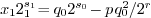
2.2.1.Modular product
Let be an integer such that  .
The remainder
.
The remainder  can be obtained as follows:
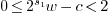
-
Decompose into
 and
and
 such that
  , with
  , and compute
  . From
  it follows that
  . So
. So  has size at most
  , and we
have
, and we
have  .
.
-
Compute
 . From the definition of
  we have:
 .
.
It follows that
 .
.
-
Let
 . From we deduce
that
. From we deduce
that  . It thus suffices to substract at most
 times
times  to obtain .
In general we can always take  and
and  , so that
  . For when
  , it is better to take
  and so that
  . Finally, for when
 one can take
  and
and  so that
  . These settings are
summarized in the following table:
. These settings are
summarized in the following table:
|
|
 |
|
|
 |
 |
|
|
 |
 |
|
|
 |
 |
 |
In these three cases remark that the integer
has size at most  .
.
It is clear that the case leads to the fastest
algorithm since step 3 reduces to one substraction/comparison that can
be implemented as min within type C
alone. A special attention must be drawn to when
within type C
alone. A special attention must be drawn to when  ,
that corresponds to
,
that corresponds to  : we must suppose that
  is indeed computed within an unsigned int type,
hence is sufficiently large to ensure
is indeed computed within an unsigned int type,
hence is sufficiently large to ensure  and
and  , hence the correctness of the algorithm.
2.2.2.Numerical inverse
Let us now turn to the computation of the numerical inverse of . The strategy presented here
consists in performing one long division in C followed
by one Newton iteration. Let  be the numerical
inverse of , normalized so that
be the numerical
inverse of , normalized so that  holds. Let
  denote the initial
approximation, and
denote the initial
approximation, and  be its Newton iterate
  . If
. If  for some positive
integer
for some positive
integer  then it is classical that
  with
with  .
.
Under the assumption that  , we can compute a
suitable as the floor part of
, we can compute a
suitable as the floor part of  by the only use of operations within base type C. In
other words we calculate
by the only use of operations within base type C. In
other words we calculate  as follows:
-
If
 then
then  is obtained
by means of one division in C.
is obtained
by means of one division in C.
-
Otherwise
 . We decompose
into
. We decompose
into  , with
  . Note
that
. Note
that  . Within C perform the
long division
. Within C perform the
long division  . By multiplying both side of
the latter equality by
. By multiplying both side of
the latter equality by  we obtain that
  . From and
  , we easily deduce since
  and
and  .
.
The computation of  , that is the floor part of
 , then continues as follows:
-
From the definition of , one can write:
 . We thus compute
  and the
ceil part of
and the
ceil part of  in order to deduce the floor
part
in order to deduce the floor
part  of
of  . Note that
fits C.
. Note that
fits C.
-
From the above inequalities it follows that
 .
We thus obtain
.
We thus obtain 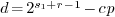 < 2p. If
  then return
  else return
  .
.
Finally, is deduced in this way:
-
Set as (
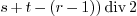 , and compute
as just described.
, and compute
as just described.
-
Note that
 . If
. If  +1=
+1= then
then  otherwise
 .
.
2.2.3.Modular product by a constant
Let be a modulo
integer that is to be involved in several modular products. Then one
can compute  just once and obtain a speed-up
within the products by means of the follows algorithm:
just once and obtain a speed-up
within the products by means of the follows algorithm:
-
Compute
 . It follows that
  .
.
-
Compute
 . If
. If  then
c=c+1. Return .
then
c=c+1. Return .
The computation of  can be done as follows from
:
can be done as follows from
:
-
Compute
 . Note that
  .
.
-
Since
 , with
  if and
  otherwise, deduce
 from
from  .
.
3.Further remarks
- On some processor architectures code to manipulate short int can be larger and slower than corresponding code which deals with int. This is particularly true on the Intel x86 processors executing 32 bit code. Every instruction which references a short int in such code is one byte larger and usually takes extra processor time to execute.
- Do not use char but signed char or unsigned char for the sake of portability.