![\[ f (x, y) = \sum_{0 \leqslant i \leqslant d_1, 0 \leqslant j \leqslant d_2} c_{i, j} B^i_{d_1} (x ; a, b) B^j_{d_2} (y ; c, d), \]](form_470.png)
 , defined by an implicit equation
  , where
 ![$f \in \mathbbm{Q}[x, y]$](form_468.png) . It uses the representation of polynomials in the Bernstein basis of a domain
. It uses the representation of polynomials in the Bernstein basis of a domain ![$[a, b] \times [c, d]$](form_469.png) :
:
where  is the Bernstein basis in degree
  , on the interval
 ![$[a, b]$](form_183.png) . The polynomial
. The polynomial  will be represented by its control coefficients
  and the domain . It can be subdivided by applying the de Casteljau algorithm, in the
  and
and  direction.
The subdivision algorithm is based on a criterion for detecting the regularity of the curve , in the domain .
Definition: We say that a domain ![$D = [a, b] \times [c, d]$](form_474.png) is regular for , if its topology in is regular for , if its topology in  is uniquely determined from the intersection points of , with the boundary is uniquely determined from the intersection points of , with the boundary  of . of . |
Here is a property that we use to detect regular domains:
Proposition: If  (resp. (resp.  ) in , then is regular for . ) in , then is regular for . |
The test is implemented by checking that the control coefficients of  or on D have a constant sign, which implies the previous proposition.
|
Algorithm: Subdivision algorithm for implicit curves.
input:
. |
void topology::assign(point_graph<C> & g, MPol<QQ>& p,
           TopSbdBdg2d<C> mth,
           C x0, C x1, C y0, C y1);
g of type topology::point_graph<C>, which is isotopic to the curve defined by the polynomial p, in the box ![$B = [x_0, x_1] \times [y_0, y_1]$](form_485.png) . The coordinates of the points in
. The coordinates of the points in g are of type C. The implementation is designed for C=double.p are rational numbers. During the computation, they are rounded to double number types. If the topology in the box can be certified from this approximation, a graph of points connecting the intersection of the curve with the boundary of  is computed. Otherwise the box is subdivided into
  subboxes and the test is applied recursively.
 specified by the class
 TopSbdBdg2d<C>. The default value is  .
.synaps/topology/TopSbdBdg2d.h, TopSbdBdg.![]()
![]()
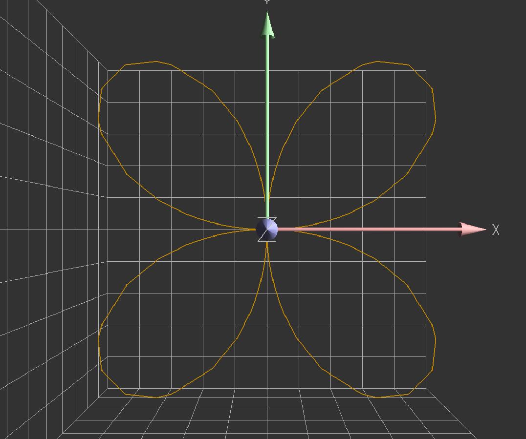
#include <synaps/topology/TopSbdBdg2d.h>

int main(int argc, char** argv)
{
  MPol<QQ> p("x^6+3*x^4*y^2+3*x^2*y^4+y^6-4x^2*y^2");
  topology::point_graph<double> g;
  topology::assign(g, p, TopSbdBdg2d<double>(),
                   -2., 2.1, -2.2, 2., 2);
}
Here is a picture of such output:
![$f (x, y) \in \mathbbm{Q}[x, y]$](form_479.png) defining the implicit curves
defining the implicit curves  and a domain
 ![$D = [a, b] \times [c, d] \subset \mathbbm{R}^2$](form_481.png) .
. with
with  ;
; to get the topology of