![\[ \left\{ \begin{array}{l} f_1 (x_1, \ldots, x_n) = 0\\ \vdots\\ f_s (x_1, \ldots, x_n) = 0 \end{array} \right. \]](form_367.png)
We consider here the problem of computing the solutions of a system
in the case where such a system has a finite number of solutions in  . The method developped in [PhT02] is implemented here. It proceeds in two steps
 .
. is the following:
From this normal form , we deduce the roots of the system as follows. We use the properties of the operators of multiplication by elements of 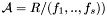 . For any
  , we define
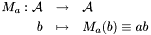
We also consider its transpose operator
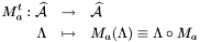
The matrix of  in the dual basis of a basis
  of
of  is the transpose of the matrix of
  in .
in .
Our approach to solve polynomial systems is based on the following fundamental theorem:
Theorem: [AuSt88] [BMr98]Assume that  . We have . We have
|
Since  is a basis of , the coordinates of
  in the dual basis of
  are
are  . Thus if contains
  (which is often the case), we deduce the following algorithm:
simple roots)}
Let such that  if
if  (which is generically the case) and be the multiplication matrix by
  in the basis
  of .
of .
 of
of  .
. with
with  , compute and return the point
  .
.template<class C> Seq<VectDse<std::complex<double> > > solve(L,Newmac<C>);
C is the type of coefficient in which we want to compute the normal form,synaps/msolve/Newmac.h.![]()
![]()
#include <synaps/arithm/gmp.h>
#include <synaps/mpol.h>
#include <synaps/base/Seq.h>
#include <synaps/msolve/Newmac.h>

typedef MPol<RR> mpol_t;

int main (int argc, char **argv)
{
  using namespace std;

  mpol_t p("x0^2*x1-x0*x1-1"), q("x0^2-x1^3-1");

  std::list<mpol_t> I; I.push_back(p); I.push_back(q);

  cout << solve(I, Newmac<RR>())<<endl;

  //| [ (0.421134,0.779225) (-1.15111,0.166259) ]
  //| [ (0.421134,-0.779225) (-1.15111,-0.166259) ]
  //| [ (1.24525,-0.588209) (-0.0526987,1.13817) ]
  //| [ (-0.424222,0.478962) (0.405487,0.957865) ]
  //| [ (1.24525,0.588209) (-0.0526987,-1.13817) ]
  //| [ (-0.424222,-0.478962) (0.405487,-0.957865) ]
  //| [ (1.5648,3.86247e-19) (1.13148,8.13152e-19) ]
  //| [ (-1.04912,-1.30962e-18) (0.465166,-1.41031e-19) ]

  // The result is a sequence of vectors with  coefficients of type
  // complex<double>. The columns correspond to the coordinates
  // of the roots (here x0, x1). The rows correspond to the roots
  // of the system (here 8 roots, with 2 which are real).
}
![$R = \mathbbm{R} [x_1, \ldots, x_n]$](form_418.png) connected to the constant polynomial
connected to the constant polynomial  {{Any monomial
  is of the form
  with
with  and some
  in
in  .}}. If
  is the vector subspace generated by
  ,
,  is a linear map such that
  the maps
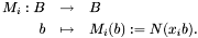
 ,
,  .
. , where
  is the ideal generated by the kernel of
  is canonical.
  ) are
) are  .
. are (up to a scalar)
  .
.