Principle

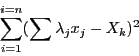
We consider here a special occurrence of quadratic equations that describe distances between points in an $n$ dimensional space. Each equation $F_k$ in such system may be written as:

$$\sum_{i =1}^{i =n}(x_i-x_j)^2+L_k=0$$

where $x_i$ are unknowns (representing coordinates of points) and $x_j$ may be unknowns of constants. A special occurrence of unknowns are the virtual points: the coordinates of these points are linear combination of the coordinates of the points that are defined as the unknowns of the system. To illustrate the concept of virtual points consider 5 fixed points on a rigid body in the 3-dimensional space. The coordinates of any of this point may be expressed as a linear combination of the coordinates of the 4 other points (as soon as these point are not coplanar). The concept of virtual points has been introduced to allow a decrease in the number of unknowns but also because without them distance equations will be redundant and consequently the jacobian of the system of equations will be singular at a solution thereby prohibiting us of using the tests (such as Moore or Kantorovitch) that allows to determine that there is one unique solution in a given box.

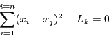
Equations involving virtual points may be written as:

$$\sum_{i =1}^{i =n}(\sum \lambda_j x_j -X_k)^2$$

where the $x_j$ are unknowns and the $X_k$ unknowns or constants. Clearly system involving distance equations are of great practical interest and ALIAS offers a specific algorithm to deal with such type of systems.

The method proposed in ALIAS to solve this type of systems is based on the general procedure using the gradient and hessian. A first difference is that it is not necessary to provide the gradient and hessian function as they are easily derived from the system of equations. Note also that due to the particular structure of the distance equations the interval evaluation leads to exact bounds. Furthermore the algorithm we propose uses a special version of Kantorovitch theorem (i.e. a version that produces a larger ball with a unique solution in it compared to the general version of the theorem), an interval Newton method, a specific version of the simplex method described in section 2.14 and a specific version of the inflation method described in section 3.1.6 (i.e. a method that allows to compute directly the radius of a ball around a solution that will contain only this solution). In addition two simplification rules are used:

• as each function is a sum of square term each of them involving different unknowns we verify if the interval evaluation of the term has a positive part (in the opposite case the current box is discarded) and we may update the unknowns so that the negative part of the term is reduced (this is basically an application of the concept of 2B-consistency). Hence the procedures described in section 2.17 should not be used for distance equations.
• based on the triangle equation: each subset of equations describing the distances between a set of 3 points is detected and the algorithm verify if the triangle equation is satisfied and, in some cases may update the boxes.

The algorithm returns as solution either boxes that satisfy Kantorovitch theorem and therefore are reduced to a point or boxes such that the function evaluations include 0 and have a width lower than a given threshold.