Accuracy Analysis and System Validation
In
this chapter, an error analysis of the system will be carried out. Since
many alternatives were presented for each of the problems encountered,
only the most useful will be fully addressed.
Acquisition Error
The
acquisition system represents the largest source of error, its different
parts are addressed in the following paragraphs.
Calibration Error
Depending
on the calibration technique, the precision and accuracy of the system
varies widely. The main difference is in between robust calibration and
classical calibration. Each class of techniques is herein addressed.
Robust techniques
Tsai's
algorithm (Tsai 1987) will be used to represent this class of calibration
techniques. Assuming the procedure exhibits acceptable convergence (see
3.4.2.2), the obtained results will at most be as accurate as the model
of the camera. In other words, the computational effort carried out by
the algorithm is only to insure the convergence of the model parameters,
it does not guarantee that the readings obtained using these parameters
will follow the actual results. Therefore, if any of the following two
cases is present, the obtained parameters will not produce accurate measurements.
The
parameters converged to a local minimum.
The
camera model, along with the embedded uncertainties do not translate the
actual functioning of the camera.
The
first case can be accounted for by using different minimization techniques,
such as the parameterization technique introduced by Zhang et al.
(1995). The second case can be avoided by using a camera with good performance,
or by introducing any missing terms into the model, as was previously proposed
in section 3.4.2.2 for the case of the radial-lens distortion. Nevertheless,
there will always be some minimum requirements for the camera to behave
consistently. These cannot be specified apriori, but a camera can be tested
as to whether it will produce consistent results for a certain calibration
technique. The camera used in the experimentation was unfortunately not
consistent, mainly due to the low performance of its lens, as it was originally
designed to be used as a web camera.
Classical Techniques
The
classical techniques are as precise as the positioning instruments used,
and as accurate as the given camera specifications.
Positioning
instruments can have very high precision and repetabilities. A very good
example of such a device is the FaroArm (Faro 1998), which is a six-degree
of freedom positioning tool that can attain an accuracy of 0.178mm. Moreover,
it offers many desirable features such as a very low sensitivity to noise,
high reach, built-in DSP, etc...
On
the other hand, the effect of camera specifications can be illustrated
by the following example. If the focal length is given with a ±1%
maximum error, then the depth is calculated as:
 (6.1)
(6.1)
where
f
is the scaled focal length, the scale factor being typically of the order
of 100; therefore, the error in pixels will be ±1.
Calibration Data
Since
all calibration procedures require the reading of some set of calibration
data, the accuracy of the system that provides these points should be addressed.
In the case of this work, all calibration data were obtained using the
get105point procedure (see appendix A). In general, calibration points
are acquired by isolating certain feature of the image, typically crosshairs
obtained by edge detecting or dots obtained by centroid fitting.
The
first alternative is the most widely adopted, were a calibration grid is
usually used as shown in Figure 6.1. The second alternative, which consists
of localizing points, has recently been given more attention, because subpixel
localization can readily be applied to it.
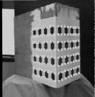
Figure 6.1 A typical calibration
grid for use with edge and point detection
Subpixel
accuracy can be achieved if sufficient assumptions are made about an image
(Hitchcock and Glasbey, 1997). For instance, Heikkiliä and Silvén
(1996) and Welch (1993) estimate the center of the calibration points calculation
the centroid of the corresponding ellipse. Figure 6.2 shows a calibration
point and its fitted contour, the contour is then interpolated into an
ellipse and its centriod calculated.
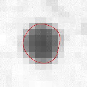
Figure 6.2 Centroid estimation
However,
although the above algorithm claims to localize the calibration point at
subpixel accuracy, it should be noted that the readings of the contour
fit (Figure 6.2) are still digital and can only be acquired at measuring
precision (camera resolution). Therefore, the actual accuracy of the system
is difficult to estimate.
The
proposed algorithm recognizes point centers up to measuring precision based
on their respective brightness, as shown in Figure 6.3, which represents
of a black disk viewed at an oblique angle.
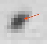
Figure 6.3 The red arrow
points to the darkest pixel. The brightness and contrast of the picture
were adjusted to make its features more distinguishable.
The
only requirement for the proposed procedure is to have the dots small enough,
typically up to 5 pixels along the major axis, unless the shape shown in
Figure 6.4 is used. This shape allows the diffusion of the colors inside
the point (see sections 4.3.1 and 4.3.2). The resulting benefits are evident
from Figure 6.5.
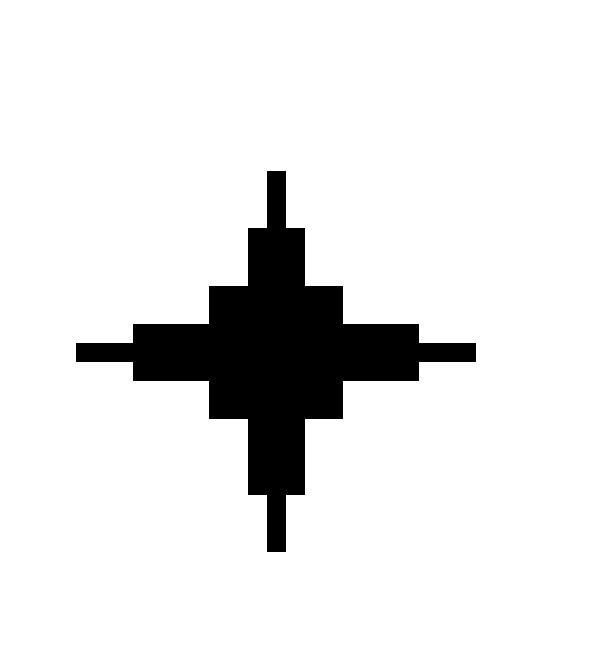
Figure 6.4 Shape for calibration
point.
Figure 6.5 The shape of Figure
6.4 gives a good estimate of the center of the calibration point even for
bigger targets. The image has been retouched for clarity.
The
error introduced is equal to the quantization error, which is a zero-mean
uniformly distributed error, and has a standard deviation of 1/12 (Kreyszig
1988). The main advantages of the algorithm over the previous one is its
simplicity, which makes it computationally more efficient.
Correspondence Error
The
correspondence algorithm was implemented in a way to eliminate the matching
of any ambiguous pair of points. In other words, the possibility of obtaining
a false match is almost completely eliminated by dramatically lowering
the number of delivered matches when the acquisition conditions are not
favorable. It should be noted, however, that a good performance of the
correspondence algorithm is insured if the calculations of the fundamental
matrix are accurate, which in turn depend on the calibration procedure.
Depth Calculation Error
The
error from depth calculation is mainly due to the quantization error in
the disparity. Referring to equation 6.1, and since the maximum error in
the disparity is 1 pixel, this lead to the following expression of the
relative error:
 (6.2)
(6.2)
where
z
and
z'
are the two possible values of the depth, and
d is the corresponding
disparity. For wide base stereo systems, the disparity is close to one
half of the camera resolution. For the case of a 640´480 image, this
error is around 0.5%.
Matching Error
The
error introduced by storing and manipulating the data in a Grid-Model will
next be addressed.
Grid-Model Error
As
mention earlier, the error introduced from representing the CT cross sections
with the Grid-Model is equal to zero with respect to the CT image. However,
the nature of the acquired set of 3D points will not follow the Grid-Model
as closely; therefore, some interpolation scheme will be in order. Different
interpolation techniques exist for fitting the data, the most commonly
used are the nearest neighbor, bilinear and bicubic interpolations. The
difference between them is straightforward and is shown in Figure 6.6,
where the original data is interpolated over a finer grid using the above
mentioned interpolation techniques.
Figure 6.6 The different
interpolation modes
Clearly,
the bicubic interpolation delivers smoother results, which in the case
of the vertebra would better approximate the bone surface. The error normally
introduced by bicubic interpolation is the following:
 (6.3)
(6.3)
where
e is the error, Dx is the step size and k is a constant.
Equation
6.3 is valid for uniformly spaced initial data, such as the one used in
Figure 6.6. However, the acquired image will not be uniformly distributed,
and equation 6.3 will only approximate the error introduced.
Transformations Error
Each
transformation, depending on the way it is implemented will introduce a
certain error in the transformed model. In the next paragraphs, the effect
of each transformation will be considered; however, the two following observations
are first in order:
The
transformations are only performed on the CT model.
The
transformations are always performed starting from the zero state; therefore,
there will not be any error add-up.
Translation
The
translational movements do not introduce any error to the model, which
is easily concluded when considering Figure 5.4, provided the increments
are integers.
Yaw and Pitch
The
worst case situation of a 45° tilt will be considered, as shown in
Figure 6.7, where the black line represents the ideal tilt.
Figure 6.7 Error introduced
by yaw and pitch transformations
This
type of error is well know in computer graphics, a quick estimation of
which for a 512´512´52 image is the following:
 (6.8)
(6.8)
Roll
The
error of roll movement corresponds to the interpolation error introduced
when re-indexing the Grid-Matrix. Recall that the procedure for the roll
transformation is:
Calculate
polar coordinates.
Add
the roll value.
Re-index
the entries of the Grid-Matrix based using a nearest neighbor interpolation.
The
nearest neighbor interpolation error, which may be treated as the quantization
error introduced in 6.1.1.3.
Validation Steps
Throughout
the intervention, several validation indications should always be presented
to the operating crew. The following sections list these indications and
evaluate their significance
Visualization
Good
visualization of the different phases of the procedure are important for
reinsuring the surgeon. The following elements should imperatively be monitored:
A
3D model of the acquired data before and after storage in Grid-Model.
The
two Grid-Models of the acquired data and the CT cross-sections during the
matching.
The
desired position of the screws
The
actual progression of the drilling operation
Moreover,
it may show useful to include some additional steps, such as the recognition
of calibration data.
Indicators
The
two main indicators are the standard deviation for calibration, and the
matching quality indicator. The former depends on the calibration method
used, and its significance has already been discussed accordingly. The
validation factor is defined as follows:
 (6.9)
(6.9)
where
the above terms have been introduced in section 5.2.2.
Good
values of the matching validation factor are above 75%.