Model Matching
To
successfully register acquired images of the vertebra bone with respect
to the CT cross-sections, surface matching has to be carried out. Moreover,
the matching procedure must have the following characteristics:
Precision:
to allow an accurate localization of the surface.
Robustness:
to allow for a margin of errors in the acquisition system.
Computational
efficiency: to allow near real time implementation. For the surgeon in
the operating room, the proposed procedure must not add dead time to the
surgical intervention. The registration must be done within an estimate
time of 20 minutes.
The
above requirements will next be refined, and an implementation of a matching
algorithm will be presented.
Difficulties
The
main problem when dealing with medical images is the large data size, which
makes the storage and manipulation difficult.
Storage
Typically,
for an operation such as the pedicle screw insertion, the patient's spine
is scanned with a high resolution, 1024 by 1024 pixels of 1mm thickness
cuts, and 0 spacing between them. Three vertebra (approximately 20 cm)
would require 1024?1024?200 bytes of storage (200 Mbytes), assuming all
operations needed on the image can be handled by the minimal 8-bit integer
type. Clearly, manipulating two 200 Mbytes models on a medium sized machine
is not feasible in a near real-time fashion.
Computational Complexity
Many
sophisticated refinements are constantly being made to improve the quality
of surface matching. These additions however would inevitably increase
the overall complexity of the system. In the context of robotic surgery,
such add-hock solutions cannot be accepted.
Conceptual Modeling
The
proposed algorithm relies on the following representation of 3D data (thereafter
referred to as Grid-Model): Each point will be represented by a 1 in one
or more 3D matrices originally filled with 0's, as illustrated in Figure
5.1.
Figure 5.1 3D representation
of data, the colored cubes represent a value of one at indexes equal to
their coordinates, the rest represents the zeros.
Two 3D Matrices
In
the case of CT data, this representation conserves the accuracy of the
system if the following conditions are met:
The
dimensions of the matrices are at least equal to that of the CT image.
The
number of filled matrices is the equal to the number of CT cuts.
Any
spacing between the cuts must be modeled by an appropriate number of zero
matrices, as illustrated in Figure 5.2.
Figure 5.2 If 9 cuts
are made with 2mm thickness and 10 mm spacing, then 4 empty matrices have
to be inserted between each filled pair.
Correlation
To
correlate the two models, the two 3D matrices are overlapped, and a term-comparison
is used:
A
match is counted when two 1's are in the same grid position.
An
error is counted when a 1 and a 0 are in the same grid position.
The
total number of matches, and that of error are normalized and used both
as indicators of the quality of the fit. Figure 5.3 depicts an example
over a single cut.
Figure 5.3 When comparing
a green cut with a blue cut, the overlapping brown square are counted as
matches, and the rest of the colored squares as errors.
Different
combinations can now be attempted to formulate the matching criteria, an
example of which is the as follows:
criterion = (match)2
- (error)2 (5.3)
Rotation-Translation
Originally,
each model is centered in its 3D grid, with the two grids being of equal
size. A transformation is then applied to one of the models before it is
correlated with the other one. Either-one of the models may be used as
long as the choice remains consistent and only one model is always moved.
Moreover, each grid must incorporate enough clearance to allow the model
to be moved without being discarded. Therefore, the use of the CT scans
as the moving model would be preferable, because the acquired model may
be surrounded by noise, making clearance estimation confusing. Finally,
the roll, pitch, and yaw coordinates will be used for rotational movements.
Translation
Translation
in the x, y, or z directions corresponds to shifting all the ones according
to the grid x, y, or z directions respectively. Figure 5.4 shows two models
with a 10-unit translation in the x direction between them.
 Figure
5.4 The two models are shifted by 10 units in the x direction.
Figure
5.4 The two models are shifted by 10 units in the x direction.
Pitch and Yaw
The
procedure for performing a pitch or yaw rotation is carried out can best
be described by Figure 5.5, which shows a filled Grid-Model tilted incrementally
with a shearing motion by 1,2...,6 units.
Figure 5.5 A Face view of
a filled Grid-Model incrementally pitched.
Yaw
and pitch values used the above transformations are related to the actual
angles by:
 (5.1)
(5.1)
where
y
is the true yaw or pitch angle, n is the number of cuts, and p is the yaw
or pitch value used in the algorithm.
Roll
Rolling
is done by transforming to polar coordinates, adding the roll angle, and
reverting back. Figure 5.6 shows a front view for a rotation of 25°.
Figure 5.6 A front view of
a 25° roll.
Model Implementation
Aspects
of the implementation of the Grid-Model under MATLAB® (see Appendix
C for a complete listing) will next be addressed.
Storage Problem
Storage
requirements can be reduced using the two following properties of the data
and the Grid-Model:
The
second property suggests the use of sparse matrices to store the data.
However, three-dimensional sparse matrices are not supported in commercial
programming environments. An attempt to model 3D sparse matrices was presented
by Hemker and Zeeuw (1993), but their work remained as a prototype for
PASCAL structures and FORTRAN. In addition, sparse 3D matrices do not make
use of the first property, and would thus be at most 12.5% (1 bit out of
eight used) efficient in terms of storage.
The
proposed implementation represents each 52 cuts in a single floating point
2D matrix (thereafter referred to as Grid-Matrix), where the binary representation
of each entry will correspond to the points in the z direction. For example,
the entry 132 (0...001000010) in columns 56 of row 45 will mean that there
are tow points at [45 56 4] and [45 56 128]. Moreover, the Grid-Matrices
can be made sparse to account for the extra clearance that has to be introduced
to allow for grid movement. Returning to the example of 5.1.1, the 200
cuts would now need 1024?1024?4 bytes, or 4 Mbytes in full matrix form,
and at most 1 Mbytes in sparse matrix form.
Correlation
The
matches and error are counted by applying a bit-wise AND and XOR operator
respectively on the pairs of matrices. Bit-wise AND is implemented as a
mex file under MATLAB, which is an executable C-code file. The correlation
procedure was written in MATLAB, but would be more efficient if written
directly in C. As an illustration, consider the following Grid-Matrices
that hold two 2x2x8 Grid-Models:
(5.3)
 (5.4)
(5.4)
The
corresponding Grid-Models are shown in Figure 5.7.
Figure 5.7 Comparing A (red)
with B (blue): The green dots are matched values and the yellow dots are
errors.
The
matches M and errors E are calculated as:
 (5.5)
(5.5)
 (5.6)
(5.6)
The
number of ones in M and E can now be calculated, giving 9
matches and 3 errors.
A
Final consideration is in the method the number of binary ones are extracted
from each entry in M and E. The usual approach would be to
test for each bit separately, yielding an efficiency of O(52n),
where n is the number of entries. Clearly, this is not acceptable.
The proposed solution is to store a form with its entries equal to the
number of ones of its index. The first eight terms of such a matrix would
be:
 (5.7)
(5.7)
The
efficiency of this method is equal to the indexing efficiency of the language,
and is therefore maximal. However, the size of the proposed matrix would
grow to 252-1. A good compromise between speed and storage is
to divide each entry in four 13-bit numbers, the required matrix would
then occupy 65 Kbytes only.
Rotation-Translation
Although
the proposed implementation of the Grid-Model is efficient in terms of
storage, the implementation is not usable if the efficiency of the translation
and rotation are not time efficient.
Translation
A
translation in the X or Y directions, would simply be the re-indexing of
the corresponding Grid-Matrices. The efficiency for such an operation is
clearly optimal
Yaw and Pitch
Tilting
the Grid-Model by t is equivalent to dividing the Grid-Model to t parts,
then shifting each part by 1 to t/2 depending on how close it is to the
center. If t is even, the central part will not move.
The
division of the Grid-Model can be achieved by multiplying with an appropriate
mask of 1's. For example, isolating the lower fifth part is done by applying
bit-wise AND of binary
0000000000000000000000000000000000000000001111111111
to
all the entries.
The
shift of each entry would now correspond to a translation in the X direction
for a pitch angle, and in the Y direction for a yaw angle. Finally, the
t parts are recombined using bit-wise OR. The efficiency of the algorithm
is linearly proportional to t and the size of the matrix.
Roll
Unfortunately,
the roll of the matrix cannot be approximated by some set elementary movements,
because of the high distortion it introduces to the image, and therefore
no approximation mask can be convoluted with the Grid-Matrix. This would
mean transforming each matrix entry to polar coordinates, manipulating,
calculating the new Cartesian coordinates, and then interpolating a new
position. To save time, all the calculations for the new rotated coordinates
are performed off-line and stored in numbered matrices. When a roll operation
is invoked on a certain matrix, a reordering of its elements will be carried
out according to the appropriate roll matrix. As an illustration, a 6 by
6 roll matrix for 45° is shown:

The
interpolation used is the nearest neighbor, which is the fastest interpolation
scheme. The distortive implications of this type of interpolation will
be discussed, along with the other effects of the transformations in chapter
6.
Search Space
The
search space of the matching algorithm represents the different transformations
that may be carried out in order to reach the goal: a fit between the two
models. The next paragraphs contain a description of the search space using
the Grid-Model approach.
Absolute Search Space
A
brute force conception of the search space is to start from a zero state,
denoted by [0 0 0 0 0 0], where the six zeros correspond to zero values
of the roll, pitch, yaw rotations and x, y, z translations, respectively.
Each new node will then be represented by a variation of the above parameters,
corresponding to the appropriate transformation. An example of a reduced
portion of the space is shown in Figure 5.8.
Figure 5.8 A sample of the
search space
If
the roll, pith, and yaw are constrained to ±45°, and the x,
y, z translations to ±45 units, then the possible values correspond
to any combination of column entries from the matrix:
such
as
[24 -12 41 0 20 13]
The
span (size) of such a space is equal to:
Alternative Search Space
A
more efficient and intuitive search space can be constructed using the
node shown in Figure 5.9, where each of the twelve arrows indicates a certain
incremental transformation.
Figure 5.9 The essential
node used in the alternative search space.
The
new search space still has the same span; however, its new diffused shape
makes it easier to "walk" it; i.e., to search for the goal position. A
sample of the alternative search space is shown in Figure 5.10. Finally,
it should be noted that the new space is a closed graph; i.e., any node
(state) can be reached from any other state.
Figure 5.10 A sample of the
alternative search space.
Search Mode
Searching
for the goal solution is done by walking the above referenced graph, starting
from the [0 0 0 0 0 0] state to reach the goal state. Figure 5.11 shows
an example of a binary search space with 5 variables; i.e., one that contains
a combination of the 32 states of:
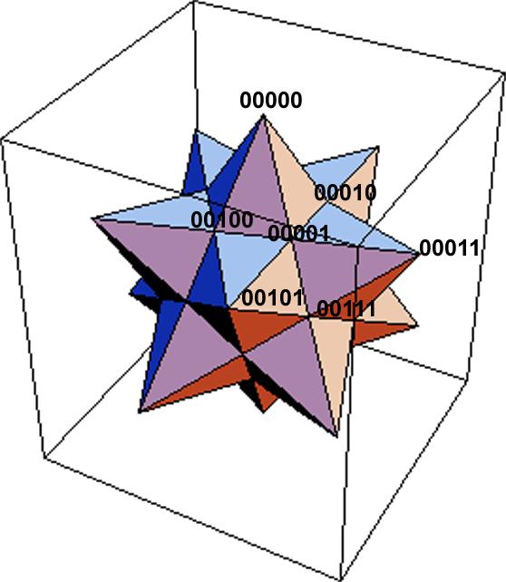
Figure 5.11 Representation
of a binary 5 variables search space with a few sample points (graph borrowed
from Mathematica®)
The
most crucial characteristic of a matching algorithm is the way it reaches
the goal. To illustrate the concept of the size of a search, consider the
goal:
[2 2 -2 1 0 2 -1]
A
breadth-first search; i.e., trying to vary all the parameters from lowest
absolute value to highest, yields:
[0 0 0 0 0 1] [0 0 0 0 1 0]
[0 0 0 1 0 0] [0 0 1 0 0 0] [0 1 0 0 0 0] [1 0 0 0 0 0]
[0 0 0 0 0 -1] [0 0 0 0 -1 0]
[0 0 0 -1 0 0] [0 0 -1 0 0 0] [0 -1 0 0 0 0] [-1 0 0 0 0 0]
[1 0 0 0 0 1] [1 0 0 0 1 0]
[1 0 0 1 0 0] [1 0 1 0 0 0] [1 1 0 0 0 0]
[1 0 0 0 0 -1] [1 0 0 0 -1 0]
[1 0 0 -1 0 0] [1 0 -1 0 0 0] [1 -1 0 0 0 0] ...
where
reaching the goal state takes at least 800 trials; therefore, although
the breadth-first approach is safest to walk such a space, because the
initial conditions are assumed to be 'close' to the goal state, it is still
time consuming.
Steepest-Hill
A
well-know solution to the goal-reaching problem in artificial intelligence
is the steepest-hill climb (Rich and Knight, 1991). As the name implies,
a steepest-hill search will always consider the most promising alternative
at each node, where the value attributed to each node is the correlation
function between the transformed CT model and the acquired one. Ideally,
such a climb results in a shortest path (optimal) to the goal. Referring
to the example at the beginning of this section, it would take 10 trials
instead of 800 to reach the desired match.
Unfortunately,
the correlation function does not give such a consistent indication of
how close the current state is to the target, as is the case for Figure
5.12, which represents a function with similar behavior. The peaks in Figure
5.12 represent high values of the correlation function.
Figure 5.12 The correlation
function exhibits many local maxima near the goal state (graph borrowed
from MATLAB®).
There
exists many classical solution to the above problem, the most commonly
used are the following:
To
increase the transformation step, to reach convergence, and then to refine
with a smaller step starting from the new state.
To
decrease the resolution of the Grid-Model, to reach convergence, and then
to refine with a higher resolution starting from the new state.
To
use more than one correlation function.
All
of the above solutions were attempted, but none showed satisfactory results,
especially in the presence of noise.
Volume versus Surface Matching
A
proposed method to overcome the problem of poor correlation is by transforming
the surfaces to be matched to volumes. The beneficial effect on the correlation
function can be visualized by examining Figure 5.13. The best transformation
for the blue cylinder to match the red cylinder is to pitch towards the
x-axis, or to slide in the directions of the y-axis. At that point, the
volume intersection clearly increases. This is not the case for surface
intersection, which is not predictable.
Figure 5.13 The volume intersection
of the two cylinder yields a better correlation than the surface intersection.
Transforming
the CT scans to a volume is clearly a simple task, performed off-line.
However, the acquired cuts which contain some noise, will not have a closed
shape. Based on the above discussion, the following final procedure is
proposed.
The
CT scans are transformed into a volume by flooding the inside of the cuts.
The
acquired image is kept as a "cloud" of surface points.
The
two models are matched using a least square correlation criterion with
a large step size.
The
step size is lowered and step 3 is repeated until the step equals one,
which corresponds to the precision limit of the model.
Perform
a constant step match of the acquired model with the original surface CT
model.
The
use of a varying step size is to accelerate even further the matching,
and can also be considered as an extra precaution against local maxima.
Moreover, a last step has been added to account for possible a false maximum
introduced by volume-to-surface matching. In other words, after the algorithm
converges with volume matching, surface matching is performed to validate
and possibly refine the macth.
An
analysis of the effect of noise on such a matching approach will be addressed
in Chapter 6. Figure 5.14 shows the CT model with gaussian noise added
to it and Figure 5.15 shows the results of matching with the original CT
model.
Figure 5.14 CT model with
gaussian noise.
Figure5.15 MATLAB® output
of matching a noisy model at [10 6 15 -12 -6 15]. The step size and current
state are shown at every instant.
The
matching was performed in 19 steps, which is even less than the predicted
shortest path of 64 using a non-varying step size. No surface match was
necessary in this case, mainly because of the well-behaved nature of the
introduced noise.