Image Acquisition
Acquiring
the 3D structure of the bone is the first step in registration. The following
sections discuss the different features of the acquisition system, stereo
vision, and the available calibration methods. Implementations of the systems
in this work will also be addressed.
The Image Acquisition System
The
image acquisition system comprises the cameras, the video capture card,
and the illumination mechanism. Figure 3.1 shows the system in the context
of the complete setup. The illumination mechanism is application dependent,
and will be discussed accordingly. The next sections summarize some of
the most important features of the acquisition system.
Figure 3.1 The image acquisition
system.
Camera Characteristics
Two
Charged Coupled Devices (CCD) cameras are used for the acquisition of the
3D structure of the vertebra. A CCD camera has the advantage of delivering
a fully digital image, with a frame rate of up to 30 per second. However,
several other characteristics influence the quality of the delivered image.
The following sections describe some of these characteristics.
Resolution and Capture Rate
The
resolution of a CCD camera is determined by the number of Charged Coupled
Devices used in it. A CCD camera may have a resolution of up to 2048x2048
pixels, as is the case of the GEN 7 by Princeton Scientific Instruments.
The CCD camera used in the experimentation is a 640x480 Creative Sharevision,
using a 514x491 CCD grid.
The
capture rate depends on the scanning frequency of the camera. In general,
CCD cameras are manufactured to reach up to 30 frames/second, which corresponds
to the maximum human-vision capture frequency. The Creative camera delivers
30 frames/second.
The Lens
The
camera lens, or apparatus of lenses, focuses the light on the CCD array
that converts it to a digital image. In CCD cameras, the lens is a major
contributor to the degradation of the fidelity of the image, because it
suffers from several defects that distort the image on the CCD array. Lens
aberration will be addressed more thoroughly in the sections 3.3.2.
Finally,
the lens needs to be focused every time the range of the target object
is changed; moreover, for the same image, it has a finite depth of focus,
where objects outside a certain range will be blurred.
Light Balancing
Several
mechanisms exist for controlling the amount of light that enters the camera,
and the way it is interpreted. In general, these mechanisms are automated
to allow a coherent amount of light into the camera. For instance, in the
camera used for this work, electronic shutters are automatically controlled
to have speeds from 1/60s to 1/15000s, enabling it to function in a wide
range of illumination conditions.
An
important mechanism when dealing with colors is white balancing, where
the camera has to be calibrated in front of a white board to maintain a
good translation of colors under fixed illumination conditions. In the
Creative camera, white tracking is done automatically for color temperatures
ranging between 2800°K and 6000°K, where the color temperature
of light is a measurement of how close it is to white light. Although this
should mean that the camera should faithfully reproduce color under illumination
conditions ranging from the incandescent lamp (2820-3000°K) to sunlight
(»5000°K), the camera fails to do so consistently. This is largely
due to the sensitivity of CCD cameras to infrared light.
Noise
As
is the case with any sensing devices, internal noise is always present
in the final output. The Creative camera insures a 46dB signal to noise
ratio, which is satisfactory for the purpose of this work.
Other characteristics
Other
characteristics may be present in CCD cameras, such as output impedance
and internal synchronization. These however have negligible effects on
the proposed 3D acquisition.
Video capture Card
Interfacing
a digital camera with the computer often needs a video capture card that
is mainly characterized by its capture rate and maximum resolution support.
In addition, the video card controls the captured image in a number of
ways, the most important of which are described next for the Thruvu®
card used in the experimentation.
Resolution and Frame Rate
The
resolution of the captured image can be customized through the card settings.
Moreover, the frame rate can be varied between 1 and 30 frames/second.
Brightness, Contrast, Hue and Saturation
The
brightness and contrast of the image can be adjusted from the card settings,
as well as the hue and saturation of the colors. Although this may easily
be accomplished using software, when specified in the card settings, it
is done by hardware and is therefore much faster.
Stereo Systems
Binocular
stereo is a simple and flexible way to obtain 3D information about a scene.
However, it is still under investigation and no standard stereo configuration
has yet been proposed. The following paragraphs present the most commonly
used stereo configurations and discuss the advantages and drawbacks of
each.
Parallel Configuration
This
is the original stereo paradigm, where depth is recovered from the disparity
between the two images, as shown in Figure 3.2.
Figure 3.2 Elementary stereo
geometry (Sonka et al., 1993). C1 & C2 are the
centers of the cameras, P1 & P2 are image points
of P.
Where
the depth is obtained from:
 (3.1)
(3.1)
where
Pr
-
Pl is the called the disparity of the image, and 2h
the distance between the camera centers, usually referred to as the baseline.
Clearly,
depth is proportional to the disparity and the focal length. Therefore,
and since the focal length is fixed, a larger disparity sensitivity will
translate into more accurate range recovery. Disparity sensitivity is limited
by the image resolution, and can only be increased if the distance between
the cameras, or the baseline, is increased. In its turn however, a wide
baseline constrains the overlap between the two images, and limits the
useful proportion of the image, affecting again the useful resolution and
decreasing the sensitivity. This makes the parallel configuration unappealing
in most applications.
Converging Configuration
In
a converging camera configuration, the overlap between the two images can
be maximized without affecting the baseline. On the other hand, converging
stereo causes more pronounced obstruction and more involved mathematical
processing. Whereas increased obstructions have to be compromised, the
mathematical problem can be worked out nearly without any loss of accuracy.
The next sections describe the processing needed for dealing with a converging
stereo system.
Parallax and Camera Rotation
The
most important subtlety when dealing with converging stereo is the difference
between parallax and non-parallax motion. The Figure 3.3 illustrates this
difference, where in the upper images the camera rotates about its center
but does not translate. The images are thus related by a plane projective
transformation, and no parallax distortion is present. In the upper left
and lower images the camera rotates about its center and translates. The
images are no longer related by a plane projective transformation, and
motion parallax is evident (Fisher 1997).
Figure 3.3 Parallax motion
(Fisher 1997)
When
converting a convergent stereo system to a parallel one, the parallax should
not be removed, in order to conserve depth information. This is usually
done by either reverting one of the cameras to a parallel configuration
by the proper rotation, or by incorporating the rotation in the disparity
equation. An example of image rectification can be found in Kang et
al. (1994), and an example of adjusting the depth equation can be found
in Young (1994), where the depth equation 3.1 now becomes:
(3.2)
Z0
is called the depth of focus, it is the distance from the straight line
joining the two camera centers and the point of intersection of the two
optical axis (Figure 3.16). The depth of focus is obtained by calibration.
Although this is the most widely used depth recovery equation, it is an
approximate result that holds as long as the disparity is small. A more
general calculation of depth can be obtained using the following equation
from Kanatani (1993):
 (3.3)
(3.3)
where
b
is the baseline vector, m and m'
are the point
vectors joining the camera centers O and
O' to the image
point P (Figure 3.4), and q is defined as:
 (3.4)
(3.4)
Figure 3.4 Depth relationship
for converging stereo
Epipolarity
A
complication introduced by converging stereo is the change in the epipolar
conditions, as illustrated in Figures 3.5 and 3.6, respectively.
Figure 3.5 Epipoles for parallel
cameras. (Text and images from Fisher, 1997)
Figure 3.6 Epipoles for converging
cameras. (Text and images from Fisher, 1997)
The
difference between the epipoles of each image should be accounted for before
any further processing can be carried out, since it facilitates the correspondence
of left and right pairs. Figure 3.7 shows the epipoles (ep1
and ep2) of a point M on the image planes PF1and
PF1,
where C1 & C2are the camera centers.
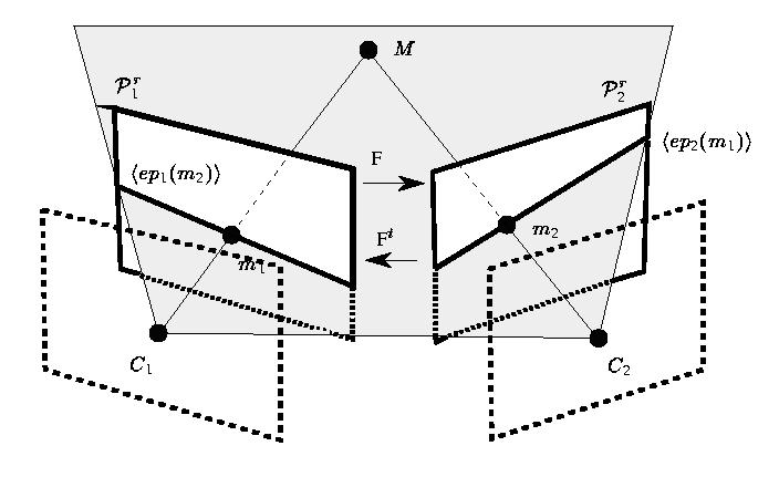
Figure 3.7 Epipolarity in
stereo vision (Robert and
Faugeras 1994)
Correspondence
The
importance of correspondence between points on each image has already been
emphasized and the classical approaches to solve the correspondence problem
have been summarized in chapter 2, their efficiency is now addressed.
Classical Correlation Method
The
main directive behind correlation methods used for stereo correspondence
is to match a certain correlation criterion for each pair of points. For
this, a window is associated around the position of each point on the second
image, where candidates for a matching pixel are evaluated. A large number
of correlation functions are currently in use, these are compared in Aschhwander
et
al. (1992), as well as several windowing mechanisms, such as the adaptive
windowing scheme described by (Kanade 1994). More sophisticated schemes
that increase robustness by accounting for occlusions can be found, such
as the one in Lan (1995).
Nevertheless,
all correlation methods are computationally demanding if an accurate match
is needed. Specifically, all points should be tested if the most of the
two images is to be used, and on each of these points, a large number of
operations has to be performed, depending on the correlation method. In
general efficiency is around O(w1w2nm) with
a considerably large overhead, where m and n represent the
image size and w1 w2 the window size. For
algorithms that make use of the epipolarity condition, the efficiency is
O(w1nm),
in which case
w1 will be is close to n/2 for
wide baseline systems.
In
the case of the spine bone, classical correlation methods have proved to
be unsuitable due to the following two characteristics of the vertebra:
The
numerous occlusions caused by its structure, and the fact that a wide baseline
system has to be used as discussed earlier, sharply decrease robustness.
The
non-uniform slopes on the vertebra body make any correlation function susceptible
to false local maxima, suggesting the use of excessively large windows.
Other methods
Correspondence
can be resolved by means other than correlation, namely, by optical flow
and Fourier transforms (Weng, 1993), and more recently complex wavelets
(Pan 1996). Optical flow and Fourier transform are badly suited to the
structure of the bone vertebra, because of the high frequency components
introduced by the irregular bone surface. Wavelets have not been explored
because of the complexity they introduce to the system.
Color Correlation
The
inability to isolate features that are easy to manipulate from the image
imposes a large computational burden, to which the following solution is
proposed: the bone will be placed under three coplanar colored light sources
pointing to it from equally spaced angles. In principle, the discrimination
of neighboring points should increase, thereby facilitating the matching
process. This method makes use of the white color of the bone and of its
very irregular contour, which allows a large color gradient on a small
surface. Figure 3.8 introduces the idea of color correlation.
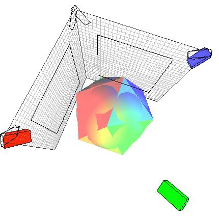
Figure 3.8 Color correlation
concept
The
next chapter is devoted to the description and analysis of the color correspondence
scheme.
Camera Calibration
Almost
all computer vision calculations rely on an ideal camera model called the
pinhole model (Figure 3.9). Moreover, a camera system is usually characterized
by its intrinsic parameters that depend solely on the camera structure,
and its extrinsic parameters that depend on its position. Calibrating a
camera is determining its intrinsic and extrinsic parameters, where the
intrinsic parameters will be used to relate the camera model to the perfect
pinhole model. The following sections discuss the different parameters
and calibration techniques.
Figure 3.9 The pinhole camera
model (from Jais 1997), where m is a point in 3D, and m' is its image.
Focal Length Calculation
The
focal length of the camera is the distance between the CCD array and the
center of the lens. Usually, it is specified in the camera data sheet;
however, two reasons stand behind the need for recalculating the focal
length:
The
focal length given in the camera specs is for the ¥ focus; therefore,
any focusing will change its value.
The
focal length is that of the lens: it is used to calculate the size of the
image projected on the CCD array, implying the need of accurate dimensions
of the CCD array (for scaling to pixels).
Consequently,
experimental computation of a value for the focal length should be addressed
before any further work can be carried out with the camera. From the depth
equation, it seems relatively easy to calculate f given a set of
points with known 3D coordinates (a grid); however, the following complications
will inevitably arise.
The
camera has to be perfectly aligned in front of the target plane on which
the grid is drawn.
The
exact distance between the target plane and the center of the length
must
be measured.
Radial-length
distortion (discussed next) should be accounted for.
Lens Aberration
To
focus the image on the CCD array, a convergent lens has to be used, and
if no other correcting lens (or system of lenses) is introduced, the image
may suffer from several distorting effects, the most important of which
is the radial-lens distortion. Figure 3.10 (a) shows a distorted image
of a grid, and Figure 3.11 (b) the same grid with radial lens correction.
Figure 3.10 Radial-lens distortion
and correction for image obtained with the Sharevision camera.
The
optical solution to this problem requires a sophisticated set of lens and
zooming equipment. The non-optical alternative is to model the distortion
and eliminate it from the image. Radial-lens distortion can effectively
be modeled by (Wolf 1983):
 (3.5)
(3.5)
where
r
is the distance between a point and the image center, r' is
the corrected distance, and k1, k2
are constants found by interpolation.
Direct Calculation
A
major difficulty in finding k1 and k2is
to obtain a good set of data to be used for interpolation. The exact focal
length has to be known in advance. However, in obtaining the focal length,
the radial-distortion was also needed. A proposed solution to this recursive
problem is to work with length ratios instead of points. Referring to Figure
3.10, the width of the small square near the center is compared to that
of the ones near the edge, this should approximate the ratio of the distances
of the centers of the squares from the image center. Figure 3.11 depicts
a radial lens correction for a set of sample points using MATLAB®.
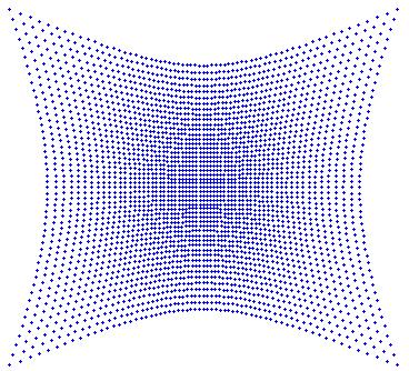
Figure 3.11 Correction for
radial-lens distortion performed on a straight grid.
An Improved Calculation
Bridges
(1997) describes a set of preliminary corrections before grid data is used
to find k1 and k2. An outline of his
approach is:
Average
several images to reduce acquisition noise
Obtain
a preliminary focal length from range approximation
Calculate
and correct for camera roll
Compensate
skewing
Calculate
and correct for camera pitch
Calculate
and correct for camera yaw
Calculate
exact focal length
Interpolate
k1
and k2
The
algorithm requires accurate knowledge of the 3D position of two additional
reference points, as shown in Figure 3.12. Moreover, only two pairs of
points are used for each calculation, and the image is totally reconstructed
before the next parameter may be calculated, resulting in a large probability
for error build-up.
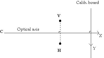
Figure 3.12 Calibration setup
Bridges (1997)
Robust Validation
An
implementation to check for the validity of the interpolated k's
is imaging a straight line on one of the borders. The corrected image should
also mirror a straight line, regardless of the direction Figure. This is
shown in Figure 3.13, where the blue square is the correction of the red
one.
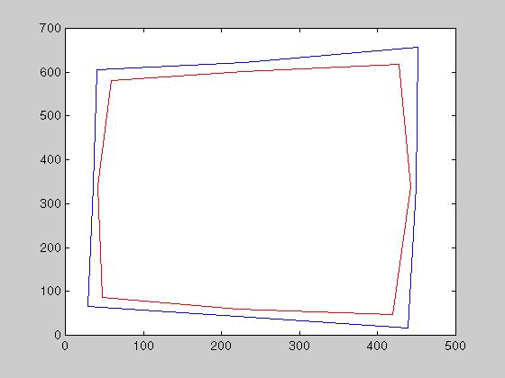
Figure 3.13 Square before
(red) and after (blue) aberration correction.
This
could further be exploited to obtain k1 and k2from
minimizing a colineation function of several point on a straight line,
the procedure is as follows:
Acquire
an image of 105 points forming 7 straight lines.
Automatically
recognize these points using their gray scale intensity, the color of their
surrounding and their approximate position.
Calculate
the square of the cross product between points on the same line as a function
of k1 and k2.
Minimize
the previous function nonlinearly for k1 and k2.
This
procedure only requires that the calibration board be rigid, and that it
spans the entire image. It is not affected by the position or orientation
of the board with respect to the camera. Furthermore, the board could even
be folded near its center, to allow for the acquisition of calibration
points from a wider focal depth, thus further decreasing the sensitivity
of the procedure to the current focal length. Such a calibration board
is shown in Figure 3.14. The algorithm used for point recognition is get105pt
(see
Appendix A), which recognizes the points based on their gray scale intensity,
and differentiates their relative position on the board from their surrounding
color.
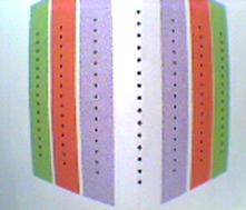
Figure 3.14 Calibration board
for radial lens distortion
Finally,
and as is the case with any non-linear optimization techniques, a good
initial guess is needed to avoid false local minima. In this case, the
coefficients obtained using the first method give consistent convergence.
The values obtained for k1 and
k2 are:
k1=
0.1397e-5
k2=
-0.1258e-11
Exact Focal Length Calculation
As
described in Kanatani (1993), an estimate of the focal length can be used
to get the exact focal length up to measuring precision. The procedure
relies on properties of the vanishing points, as shown in Figure 3.15.
Figure 3.15 The exact focal
point can be calculated as a function of the vanishing points v1 and v2.
ABCD is originally a parallelogram.
The
importance of this calculation length lies in the fact that the error caused
by lens aberration and misalignments can now be lumped in the approximate
focal length. The above procedure was tried for several sets of data, always
yielding the same value of f = 403.537.
There
are two requirements for this procedure:
A,
B, C and D should be as centered around the image origin as possible; this
would allow lumping aberration uncertainties in the approximate focal length.
The
vanishing lines have to be close enough to the image, in order not to get
a ratio of two very large numbers during the calculation.
The
procedure can be summarized as follows:
Identify
the reference camera coordinates ma, mb, mc,
and md of A, B, C, and D ([xa ya f] for A ...)
Get
the coordinates of AB, BC, CD,
and DA (AB is the cross product of A and B...)
Compute
the vanishing points mv1 and mv2 coordinates
as AB cross CD and BC cross DA.
Calculate
the exact focal point f from:
 (3.6)
(3.6)
Camera Position Estimation
Some
mathematical relations can be applied to directly solve for the camera
position. An example of such an approach has already been introduced in
3.2.2.2, where the roll, pitch and yaw of the camera are calculated with
respect to a reference board. However, the presented calculations, except
for the camera roll, assume knowledge of the distance to the center of
the board. An approach that does not use the distance from the calibration
object is next proposed.
Starting
from a parallel configuration, the two camera are tilted inwards to obtain
a convergent configuration, this stereo configuration (Figure 3.16) is
widely used because the depth calculations could be approximated by the
depth of focus equation discussed in 3.2.2.1.
Figure 3.16 Depth of Focus
Convergent Configuration (Young 1994).
Consider
a horizontal bar of known length placed between the two cameras, with the
fixation point on its center. The tilt angle could then be calculated as
described next:
Referring
to Figure 3.17, and keeping in mind that rotating a camera around an object
is equivalent to rotating that object around the camera, the dimensions
of the bar can be characterized by:
(3.7)
and
(3.8)
where
2a
is
length of the image of the bar before the rotation, and
b &
c
after a tilt of y. a and b
are the angles between
the straight lines relating the camera center to the center of the bar
and the camera center to the respective ends of the bar.
(3.9)
expanding
yields
(3.10)
and
using the fact that
 (3.11)
yields
 (3.12)
dividing
by cos(y) and simplifying yields
 (3.13)
Once
y
is obtained, the exact orientation of the cameras will be known, and depth
calculation can be carried out without any approximation.
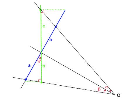
Figure 3.17 Geometry for
pitch calculation. O is the camera center, the blue bar is the bar before
rotation, the green one is after, and y is the tilt angle.
Finally,
the camera roll can also be found using a trigonometric identity described
in Bridges (1997).
The
above procedure was automated using MATLAB®, and tested on a synthetic
image and achieved an absolute accuracy of 0.1%.
Robust Calibration
By
robust calibration is meant that the calculated parameters should be acquired
in a way that insures the convergence of the model towards an ideal reference
model, usualy the pinhole model. The motivation behind robust calibration,
as is the case with most non-linear models, is that the calculated parameters
cannot be easily uncoupled from the model nonlinearities. Moreover, in
calculating parameters separately, the overall error of the system will
most likely be amplified by the error of each parameter.
Robust
calibration guarantees that the parameter will be such that the overall
system meets the ideal specifications set for it. The parameters would
converge to values that do not necessarily correspond to their true values,
but to values that balance the errors in other parameters, and account
for any un-modeled non-linearity. Practically, this approach delivers very
satisfactory results, unless active vision is used, where knowledge of
the exact parameters becomes necessary, as argued by Shih et al.
(1996).
Mathematical Preliminaries
The
following paragraphs summarize the most commonly used camera modeling schemes.
The Pinhole Model
Referring
to the Figure 3.18, the homogenous image coordinates uhand
vh
may be related to the 3D standard coordinates x, y, and z
by:
 (3.14)
where
u
= uh / s and v = vh / s, s ¹ 0.
Moreover,
and as is usually the case, if the camera coordinate system is scaled by
ku
in the u direction and kv in the v direction,
in addition to an origin translation of (u0
, v0 ),
then the previous equation would be replaced by:
 (3.15)
The
above matrix represents the mapping between a 3D coordinate system and
the image coordinate system. It only depends on the internal characteristics
of the camera, or its intrinsic parameters. Note that the camera is still
assumed to have no distortion caused by its lenses or by the misallignment
of the CCD array. Modeling these deformations is possible by incorporating
appropriate factors into the intrinsic matrix. However, these would be
limited to a first order lens aberration correction. An alternative for
correcting these aberrations has already been discissed in section 3.3.2.
The Essential Matrix
If
the coordinate system to be used is not the standard coordinate system,
and the new one is found by rotating the standard coordinate system by
R,
and translating it by t, as shown in Figure 3.18, then the
relation between the new 3D coordinates and the image coordinates is:
 (3.16)
The
second matrix is calculated from the camera extrinsic parameters,
the essential matrix is defined as:
 (3.17)
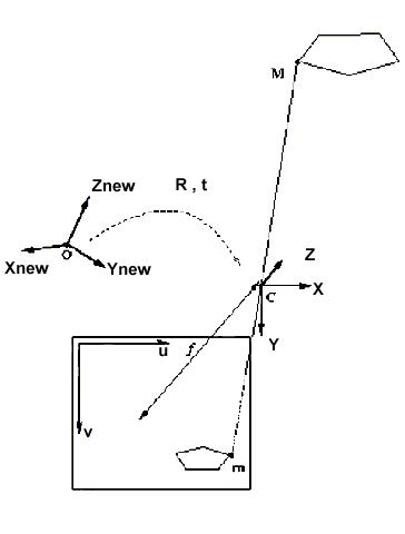
Figure 3.18 General projective
geometry (from Luong and Faugeras 1993)
The Fundamental Matrix
Finally,
and referring again to Figure 3.18, the relationships between the image
m1
of point M on the first camera, and m2 on the second camera
is:
 (3.18)
and
 (3.19)
resulting
in a relation between m1 and m2:
 (3.20)
where
the product of the three matrices is called the fundamental matrix. The
importance of the previous result lies in the fact that it could be used
to correlate epipolar points. An example of epipolar points was already
introduced in Figure 3.7, where F and FTrelate
ep1(m2)
to ep2(m1).
Implementation
In
general, camera calibration techniques may be stratified into four different
categories:
Estimating
extrinsic parameters given intrinsic parameters
Estimating
intrinsic parameters given extrinsic parameters
Estimating
extrinsic and intrinsic parameters together
Variations
in the above approaches are also possible, such as setting a number of
parameters to reduce the number of simultaneously estimated parameters.
When possible, this significantly reduces the computational burden of minimizing
a non-linear function of several parameters. Moreover, some approaches
use a calibration object of known dimension to facilitate the processing.
The following sections present some of these techniques.
Least Square estimation of extrinsic parameters
If
no calibration object is to be used, the extrinsic parameters can still
be obtained given the intrinsic parameters and a set of correspondence
points with coordinates m and m'. The coordinates
of the points are stored as [x y f], where f is the focal point.
Moreover, and since the set of point pairs is obtained by using a certain
correlation technique that inevitably introduces some error, a least square
approach is used. An example of such a scheme is developed in Kanatani
(1993):
Compute
the translation vector h from the minimum eigenvalue of G.GT,
this corresponds to minimizing in a least square sense S (m.m')2.
Define
K=-h´G
and compute the rotation matrix R that maximizes tr(RTK)
by singular value decomposition or using quaternions.
The
above procedure relies solely on the epipolarity property to estimate up
to a scaling factor the camera extrinsic parameters. It minimizes the essential
matrix introduced in 3.4.1.2, which has 8 degrees of freedoms (6 for the
rotation, 3 for the translation and 1 constrained by projective geometry).
The most important aspect of the procedure, as is the case with all robust
calibration methods, is the way non-linear minimization is implemented:
it uses variations of the generalized Moore-Penrose inverse to solve for
least square equalities. The procedure has been automated using MATLAB®,
and tested on a synthetic object shown in Figure 3.19.
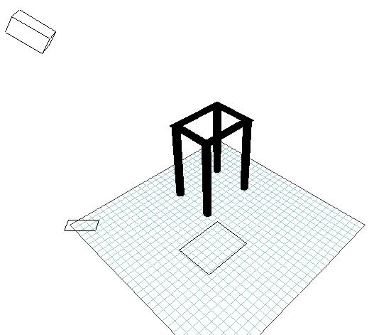
Figure 3.19 A synthetic calibration
object.
Although
the delivered results where satisfactory, the procedure is very sensitive
to noise (as confirmed by Zhang et al. 1995). Moreover, and because the
focal length is explicitly used in all the calculations, the procedure
is also very sensitive to the focal length, as shown in Figure 3.21. Finally,
the procedure does not account for the error introduced by lens aberrations,
thus the correction for radial-lens distortion had to be carried out independently
before the calibration.
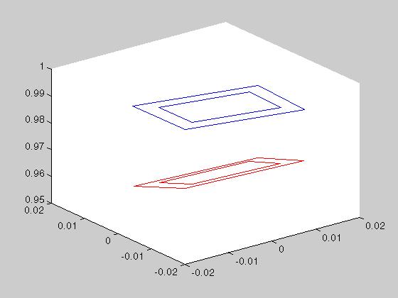
Figure 3.21 The blue square
is the top of the calibration object as seen from the first camera. The
red one is for a focal length variation of 1%.
Finally,
it should be noted that if non-linear minimization is added, the procedure
delivers better results in the presence of noise. The non-linear estimation
used is that embedded in MATLAB®, and is based on a Nelder-Med type
simplex search.
Tsai's Algorithm
An
algorithm that estimates the intrinsic and extrinsic parameters in the
same time was introduced by Tsai (1987). It minimizes in a least square
sense the fundamental matrix in for pair points from each image. A recent
implementation under MATLAB® was carried out by Heikkiliä based
on Heikkiliä and Silvén (1996). This implementation uses a
Levenberg-Marquardt optimization for non-linear minimization. The drawbacks
of the Tsai algorithm are that it needs detailed dimensions about the CCD
array, and that it models only first order radial lens distortion. A calibration
example will next be presented. Figure 3.22 shows the calibration board
with the recognized points, and Figure 3.23 the location of the points
in 3D.
Figure 3.22 Point recognition
Tsai's algorithm
Figure 3.23 The original
location in 3D for the set of points used for calibration.
The
algorithm failed to converge for several sets of calibration points. However,
when radial lens distortion was corrected before the calibration was performed,
the algorithm converged with a high standard deviation. Nevertheless, the
obtained results where totally inaccurate. The reasons for this will be
elaborated in Chapter 7.