Tumor Growth Modelling in the Brain
6. Monitoring Slowly Evolving Tumors
Most of the pediatric brain tumors as well as the majority of adult tumors are slowly evolving pathologies. Although modeling the growth of these tumors is important the slow rate of evolution brings up another question: detecting the growth. More explicitly, the clinically more relevant question is detecting the change of tumor volume between two images of a patient taken at different times. Here we describe an approach that semi-automatically performs this task using longitudinal medical images. We specifically focus on meningiomas, which experts often find difficult to monitor as the tumor evolution can be obscured by image artifacts.
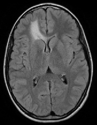
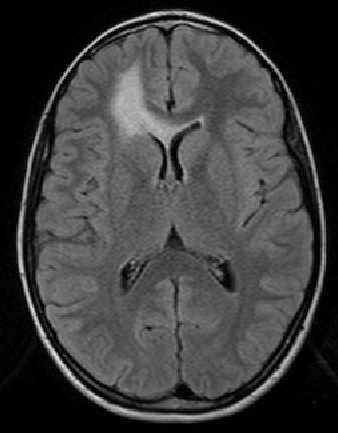
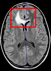
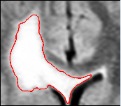
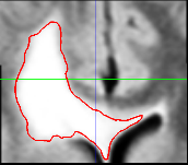
The scan on the left is taken several months before the scan on the right.
The evolution of the tumor is slow therefore detecting it becomes
a crucial question.
Meningiomas are the most common type of primary brain tumor. Most of these tumors are categorized as benign pathology that grows slowly between brain tissue and dura. To avoid the risk of surgery, neurosurgeons carefully monitor patients with benign meningiomas by having the patient regularly undergo Magnetic Resonance (MR) scanning. An expert assess the tumor growth through visual inspection of consecutive 3D scans. A precise analysis, however, is extremely difficult as slow growth is often obscured by changes in the head position or intensity profile between the two scans. We address this issue by describing a relatively fast and robust method that semi-automatically analyzes the tumor evolution.
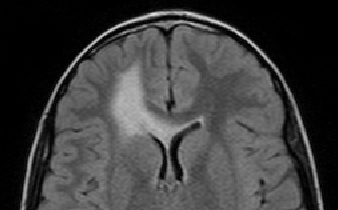
is taken several months before the scan on the right. The pose and intensity
differences makes it hard to detect small volume changes.
Our approach first semi-automatically segments the tumor in the initial patient scan. It then aligns the second scan of the patient to the first using a hierarchical rigid registration approach. Finally, it measures growth or shrinkage from these images, for which we suggest two different types of metric. Motivated by [Angelini et al. 2007], the first metric detects change through analyzing differences in intensity distributions. We differ from [Angelini et al. 2007] in that we relate the analysis to hypothesis testing. The second metric is motivated by the work of [Rey et al. 2002], which detects change by analyzing the deformation field between two scans. However, our metric returns a quantitative analysis of the differences in volume (mm3). Our approach also differs significantly from works on segmentation, such as [Prastawa et al. 2003, Liu et al. 2005] as we estimate volume change by simultaneously analyzing the sequence of scans.
6.1. The Framework
The software pipeline is composed of three steps, which are:
- tumor segmentation,
- image registration and
- change detection.
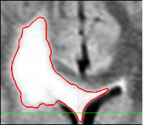
of the first scan. User selects a region of interest and
determines the right intensity. The algorithm applies
thresholding and island removal to obtain the final
segmetation.
The semi-automatic segmentation is based on a user-defined bounding box around the tumor and a lower bound of the intensities that characterize the pathology. From these indicators, the pipeline can reliably extract most of the pathology when it appears as homogeneous, bright objects in the MR images. Most of the slowly growing tumors such as low grade astrocytomas and meningiomas appear as such objects. For more complicated pathologies different segmentation techniques may be utilized and these can be plugged into the pipeline easily. The pipeline post-processes the resulting binary map by removing small islands and holes caused by the noise in the MRs. We note that the resulting map may also include part of the dura and vessels since these structures may have intensity patterns that are similar to pathology. However, because they are static, these additional structures should not substantially impact the analysis.
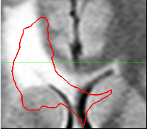
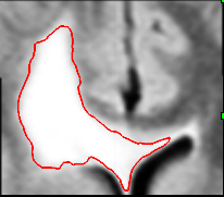

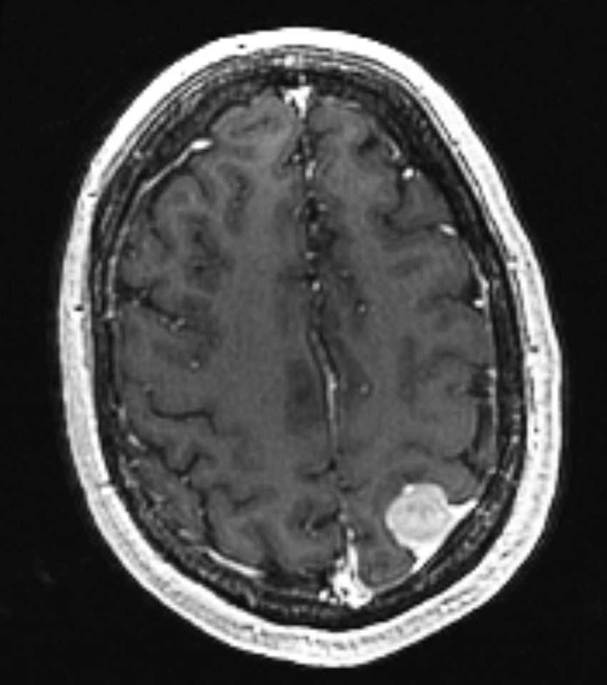
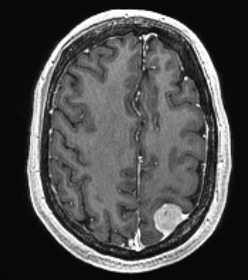
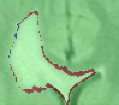
during the image acquistion. The second step in our pipeline
is to rigidly align the two scans. The image on the left
shows the bounding box and the segmentation we have obtained
from the first scan drawn on to the second scan.
Notice the misalignment. The image on the left shows
the same thing after the rigid alignment.
The second step automatically aligns the pathology of the second scan to the first. It does so by rigidly registering the scans. Now, we assume that the previous bounding box is large enough so that its coordinates also define a bounding box around the pathology in the second scan. We then accommodate partial voluming in images by increasing the resolution of both bounding boxes. Finally, the framework addresses non-linear perturbation artifacts caused by the MR acquisition by rigidly aligning the contents of the bounding boxes with each other. This results in two images where, in theory, barring temporal changes, the pathology is well aligned.
The final step of our approach measures the tumor evolution based on the initial segmentation and the bounding boxes described above. We now propose two different types of analysis for detecting the volume change.

images of the pathology in different times, in the
upper row we show these images. At this point the
images are ready to be compared for growth detection.
The image on the bottom shows a map of volume
changes obtained using the Intensity Analysis.
- Intensity Analysis: The first analysis is based on a statistical model that differentiates changes in the intensity patterns that are due to evolving pathology rather than image artifacts. In this model we first learn the intensity variability between two scans that is due to image artifacts, σart. This is simply achieved by comparing the intensity patterns in the two scans using the regions where there are no enhancement due to the tumor. Based on the learnt σart we then compare the intensity values in the scans and mark the differences exceeding σart as growth or shrinkage.
- Deformation Analysis: The second analysis is based on the amount of deformation required to map the bounding box coming from the first scan to the one coming from the second scan. We obtain this deformation field, D, by non-rigidly registering the two scans using the diffeomorphic demons algorithm [Vercauteren et al. 2007]. Using the D we can estimate the amount of volume change by two ways. The first one is to analyze the Jacobian of this field JD whose determinant provides us the volume change. The second way is to apply the deformation to the delineation of the first scan obtained using semi-automatic segmentation. Comparing the original and the deformed delineations gives the us the volume difference.
6.2. The Output
This semi-automatic framework provides the difference between the two scans in terms of mm3 and in percentage of growth. Starting from the images it can even detect very small changes in an interactive workflow. Further analysis on this respect is given in [Konukoglu et al. 2008]. After all the steps of the algorithm are completed we obtain the following picture: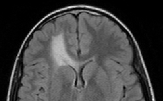
| Intensity Analysis | Jacobian Analysis | Segmentation Analysis | |
| Computed Growth | 557.4 mm3 (7.8%) | 1539.4 mm3 (21.6%) | 1555.7 mm3 (21.9%) |
using the framework explained in the previous section. The volume differences
are given in mm3 and in %.
6.3. References
- [Konukoglu et al. 2008] E. Konukoglu, W. M. Wells, S. Novellas, N. Ayache, R. Kikinis, P. M. Black, K. M. Pohl. 2008, Monitoring Slowly Evolving Tumors. ISBI, pp. 812-815.
- [Angelini et al. 2007] E.D. Angelini and J. Atif and J. Delon and E. Mandonnet and H. Duffau and L. Capelle. 2007, Detection of glioma evolution on longitudinal {MRI} studies. ISBI, pp. 49-52.
- [Rey et al. 2002] D. Rey and G. Subsol and H. Delingette and N. Ayache, 2002, Automatic detection and segmentation of evolving processes in 3D medical images: Application to multiple sclerosis. Medical Image Analysis, vol. 6, pp. 163-179.
- [Prastawa et al. 2003] M. Prastawa and E. Bullitt and N. Moon and K.V. Leemput and G. Gerig, 2003, Automatic brain tumor segmentation by subject specific modification of atlas priors. Academic Radiology, vol. 10.
- [Liu et al. 2005] J. Liu and J. Udupa and D. Odhner and D. Hackney and G. Moonis, 2005, A system for brain tumor volume estimation via {MR} imaging and fuzzy connectedness. Computerized Medical Imaging and Graphics, vol 29.
- [Vercauteren et al. 2007] T. Vercauteren and X. Pennec and A. Perchant and N. Ayache, 2007, Non-parametric diffeomorphic image registration with the demons algorithm. MICCAI, vol. 4792, pp. 319-326.